How Much of a Data Science Workflow Can Run on a GPU Today? Part 1: Accelerating Data Preparation

Many data scientists spend much of their time working with tabular data. Traditionally, these workloads have run on CPUs, which is often sufficient until an expensive operation becomes a bottleneck. Meanwhile, much of the discussion around GPUs focuses on deep learning and large language models. Today, however, GPU acceleration is available across much of the Python data science stack, allowing many existing tabular data workflows to run on GPUs with little or no code changes.

A lot of discussions around GPUs focus on deep learning and large language models. However, a lot of data scientists still spend most of their time working with tabular data where most of these workloads have traditionally run on CPUs. This is usually fine until an expensive operation becomes a bottleneck. The illustration below captures this in a lighthearted way.

Today, GPU support is available across much of the Python data science stack, making it possible for data scientists to accelerate many existing workflows with little or no code change. This reduces the time spent waiting for expensive operations to finish, leaving more time to focus on solving the actual problem.

I decided to go through a typical machine learning pipeline one step at a time to see where GPU acceleration is available today and how practical it is to use. In this series, I’ll walk through a typical machine learning pipeline one step at a time to see where GPU acceleration is available today, how much code needs to change, and when CPUs are still the better choice.

We’ll begin with tabular data processing and the data preparation tasks that are part of many day-to-day data science workflows.

Dataset and Code

Throughout this article, we’ll use the NYC Yellow Taxi Trip Records datase (CCO License), It contains millions of taxi trips collected in New York City, with information such as pickup and drop-off locations, trip distance, passenger count, fares, and timestamps. For this article, we’ll only use the first three months which gives us roughly 9–10 million rows. 

To keep the examples focused, I’ve omitted some boilerplate code and shortened a few snippets. The complete code is available here.

---

Accelerating Pandas Workflows on GPU

If your data processing pipeline is built with pandas, there are two easy ways to run it on the GPU :

• Working directly with the native cuDF API.
• Accelerating existing pandas code with cudf.pandas.

Let’s look at both these approaches.

1. Building GPU-native workflows with the cuDF API

If you’re starting a new project and want to work directly with GPU DataFrames, cuDF could be a great option. It is part of RAPIDS , NVIDIA’s open source suite of GPU-accelerated libraries for data science and analytics.

cuDF is a Python GPU DataFrame library for manipulating tabular data using a pandas-like API. So, if you’re familiar with pandas, much of the syntax will look familiar. The difference, however, is that unlike pandas, cuDF executes these operations on the GPU rather than the CPU. Something to note, however, is that while cuDF closely follows the pandas API, it is not a complete drop-in replacement, so some behaviors may differ.
Installation

If you’re using Google Colab, cuDF is already available in the GPU runtime. Otherwise, install the cuDF package that matches your installed CUDA version. 
You can check your CUDA version by running:

!nvidia-smi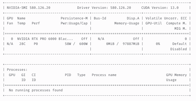

For example, if your system reports CUDA 13.x, install the CUDA 13 build of cuDF:

pip install cudf-cu13

Refer to the installation guide for the complete list of installation options and supported CUDA versions.

Loading data into a cuDF DataFrame

Loading data into a cuDF DataFrame works just like pandas. In most cases, you simply replace pandas.read_* with the corresponding cudf.read_* function. Here’s how you’d load a Parquet file using cuDF:

import cudf

taxi_url = 'https://d37ci6vzurychx.cloudfront.net/trip-data/yellow_tripdata_2023-01.parquet'

df_gpu = cudf.read_parquet(taxi_url)
df_gpu.info()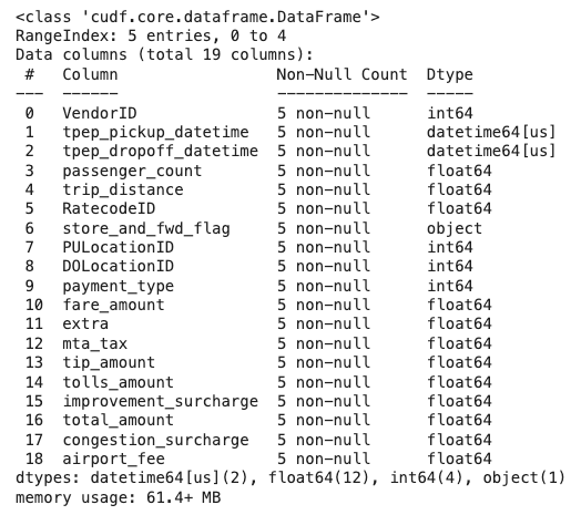

Once the data is loaded into GPU memory, subsequent DataFrame operations run on the GPU.

Working with cuDF

cuDF supports many of the same operations you already use in pandas. Here are a few common examples:

Selecting columns

trips = df_gpu[ [ "PULocationID", "DOLocationID", "fare_amount", "trip_distance", "tip_amount", ] ]

Filtering rows

high_fare = trips[trips["fare_amount"] > 20]

Creating new columns

trips["tip_percentage"] = ( trips["tip_amount"] / trips["fare_amount"] * 100 )

Summary statistics

trips.describe()

Moving between pandas and cuDF

Many data science workflows use libraries that only support pandas. You can easily to move data between CPU and GPU DataFrames using cuDF, when required.

Converting a pandas DataFrame to cuDF:

df_gpu = cudf.from_pandas(df_cpu)
print(type(df_gpu_converted))
---------------------------------------
<class 'cudf.core.dataframe.DataFrame'>

Converting a cuDF DataFrame back to pandas:

df_cpu = df_gpu.to_pandas(
print(type(df_cpu_converted))
---------------------------------------
<class 'pandas.core.frame.DataFrame'>

These conversions are useful when a downstream library only supports pandas or when you want to migrate an existing workflow to the GPU.

Comparing pandas and cuDF

To see the performance difference in practice, let’s run the same analysis using both pandas and cuDF. We’ll group the trips by pickup location and calculate the total fare amount, average trip distance, and trip count for each location.

def summarize_trips(df):
    return (
        df.groupby("PULocationID")
          .agg(
              {
                  "fare_amount": "sum",
                  "trip_distance": "mean",
                  "passenger_count": "count",
              }
          )
          .sort_values("fare_amount", ascending=False)
    )

%time summary_pd = summarize_trips(df_cpu)
%time summary_gpu = summarize_trips(df_gpu)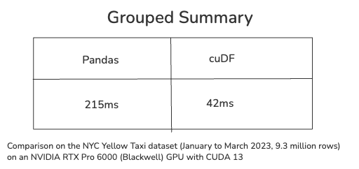

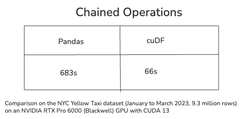
Real-world data processing rarely consists of a single operation. It often involves several DataFrame operations chained together. As another comparison, let’s run a more realistic workflow by finding the most common drop-off location for each pickup location.

def run_chain(df):
    return (
        df[["PULocationID", "DOLocationID"]]
        .value_counts()
        .reset_index(name="count")
        .sort_values(
            ["PULocationID", "count"],
            ascending=[True, False],
        )
        .groupby("PULocationID")
        .head(1)
        .reset_index(drop=True)
    )

%time result_pd = run_chain(df_cpu)
%time result_gpu = run_chain(df_gpu)

Comparing heavy aggregations

Groupby aggregations are among the most common operations in analytics pipelines and are well suited for GPU acceleration as they are expensive. Let’s benchmark a grouped aggregation across multiple columns.

def aggregate(df):
    return (
        df.groupby("PULocationID")
          .agg(
              {
                  "fare_amount": "sum",
                  "trip_distance": "sum",
                  "passenger_count": "count",
              }
          )
    )

%time agg_pd = aggregate(df_cpu)
%time agg_gpu = aggregate(df_gpu)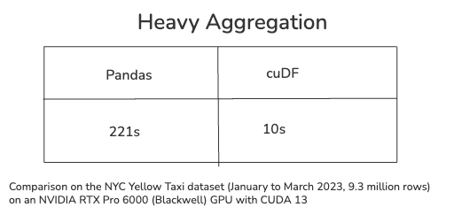

Even on this dataset, we can see a significant speedup, and on larger datasets, these aggregation workloads can benefit substantially from GPU parallelism.

---

2. Accelerating existing pandas code with cudf.pandas 

Can I speed up my existing pandas code without rewriting it?

While the native cuDF API is a great choice for new GPU-first projects, many existing data science workflows are already built around pandas and it’s a bit of work to rewrite all the code. This is where cudf.pandas comes in. It is an accelerator mode built into cuDF that helps accelerate your pandas code without any change in code.

Enable the accelerator

To enable GPU acceleration in a notebook, load the extension before importing pandas:

%load_ext cudf.pandas
import pandas as pd

For Python scripts, you can write:

python −m cudf.pandas script.py

It’s the same pandas code

We’ll use the same data and code from previous section. The only change is including the %load_ext cudf.pandas line at the top, which enables the accelerator.

%load_ext cudf.pandas
import pandas as pd

taxi_url = 'https://d37ci6vzurychx.cloudfront.net/trip-data/yellow_tripdata_2023-01.parquet'

df = pd.read_parquet(taxi_url)

summary = (
    df.groupby("PULocationID")
      .agg(
          {
              "fare_amount": "sum",
              "trip_distance": "mean",
              "passenger_count": "count",
          }
      )
      .sort_values("fare_amount", ascending=False)
)

summary

You can verify that cudf.pandas is active by printing the pandas module:

print(pd)
-------------------------------------------
<module 'pandas' (ModuleAccelerator(fast=cudf, slow=pandas))>

Every pandas operation is first attempted on the GPU using cuDF. If an operation isn’t supported, cudf.pandas automatically falls back to pandas on the CPU. 

Profiling GPU and CPU Execution

Rather than guessing which operations ran on the GPU, cudf.pandas includes a built-in profiler that reports GPU execution and CPU fallbacks.

%%cudf.pandas.profile
summary = (
    df.groupby("payment_type")
      .fare_amount.mean()
)

After the cell finishes, the profiler generates a report showing which operations ran on the GPU and which fell back to the CPU.

For more detailed analysis, %%cudf.pandas.line_profile reports how much time each line of code spends executing on the GPU and CPU.

%%cudf.pandas.line_profile
summary = (
    df.groupby("payment_type")
      .fare_amount.mean()
)

Working with Third-Party Libraries

Because cudf.pandas preserves the pandas API, many libraries that work with pandas also continue to work without modification. This means once the data has been processes, it can be passed directly to libraries such as Plotly Express without changing the downstream code.

import plotly.express as px

top10 = summary.head(10).reset_index()

fig = px.bar(
    top10,
    x="PULocationID",
    y="fare_amount",
    title="Top 10 Pickup Locations by Total Fare",
    labels={
        "PULocationID": "Pickup Location ID",
        "fare_amount": "Total Fare",
    },
)

fig.show()

This produces the same interactive visualization that we would create with a regular pandas DataFrame, but now it’s much faster. Also, since the downstream code remains unchanged, it is very easy to incorporate GPU acceleration into existing notebooks and pipelines without modifying your visualization workflow.

2. Using the Polars GPU Engine

Polars is already known for its fast DataFrame engine and Lazy API. But if you’re working with large datasets, you can also take advantage of GPU acceleration through the polars GPU engine powered by cuDF.

Like cudf.pandas, it enables accelerating existing workflows with minimal changes. When you execute a lazy query, Polars first creates an optimized query plan. If the operations in the plan are supported on the GPU, they are executed using cuDF, else Polars automatically switches to its standard CPU engine. The figure below illustrates this execution flow.

Installation

The easiest way to install the GPU engine is through the optional Polars GPU package, which automatically installs the required RAPIDS dependencies.

pip install "polars[gpu]"

or

# Direct cuDF-backed Polars engine install option for CUDA 12

pip install -q polars cudf-polars-cu12 --extra-index-url=https://pypi.nvidia.

Enabling GPU acceleration for Polars

We’ll use the same NYC taxi dataset and perform the same analysis as in the previous sections. The only difference is that we execute it with the GPU engine by passing engine="gpu" to collect().

import polars as pl
taxi_url = "https://d37ci6vzurychx.cloudfront.net/trip-data/yellow_tripdata_2023-01.parquet"
query = (
    pl.scan_parquet(taxi_url)
      .group_by("PULocationID")
      .agg(
          fare_amount=pl.col("fare_amount").sum(),
          trip_distance=pl.col("trip_distance").mean(),
          trip_count=pl.len(),
      )
      .sort("fare_amount", descending=True)
)
summary = query.collect(engine="gpu")
summary.head()

The query itself is same like a standard Polars LazyFrame workflow. The only difference is that now we are passing engine="gpu" in collect(), which tells Polars to execute the query using the GPU engine, if supported. However, If the query contains unsupported operations, polars automatically falls back to its CPU engine.

Verifying GPU execution

To check whether a query ran on the GPU, you can enable verbose mode before calling collect(). If a query cannot be executed on the GPU, Polars prints a PerformanceWarning explaining why it fell back to the CPU. You can also disable automatic fallback by passing pl.GPUEngine(raise_on_fail=True) to collect(), which raises an error if the query isn’t supported on the GPU.

unsupported_gpu_operation = (
    df_lazy
    .select(
        pl.col("fare_amount")
        .map_elements(lambda fare: fare * 1.1, return_dtype=pl.Float64)
        .alias("fare_with_markup")
    )
    .head(10)
)

with pl.Config() as cfg:
    cfg.set_verbose(True)
    fallback_result = unsupported_gpu_operation.collect(engine="gpu")

print(fallback_result)

In the example above, we intentionally use map_elements() with a Python function. Python functions are not supported by the Polars GPU engine, so this query cannot run fully on the GPU.

Scaling to multiple GPUs

The example above uses a single GPU. If you’re working with larger datasets or have access to multiple GPUs, you can switch to RayEngine with only a small change.

from cudf_polars.engine.ray import RayEngine
with RayEngine() as engine:
    summary = query.collect(engine=engine)

RayEngine automatically uses all GPUs visible to the process, allowing the same lazy query to scale from one GPU to multiple GPUs. If you’d like to learn more about how the Polars GPU engine scales across multiple GPUs, Benjamin Zaitlen has a nice blog post that walks through the concepts and includes performance examples.

Conclusion

Something I found from the benchmarks and my own experiments is that GPUs are most useful for large, data-intensive operations such as filtering, joins, groupby aggregations, and sorting. For smaller datasets, however, CPUs are often just as fast because of the overhead of moving data to the GPU involved . Thanks to libraries like cudf, we no longer need to rewrite an entire codebase to accelerate data processing and analysis. We can switch between GPU and CPU execution depending on the workload. This means we spend less time waiting for queries to finish and more time focusing on other important parts of the data science workflow. 

In the next article, we’ll move beyond data preparation and explore GPU acceleration for machine learning libraries and see how much code actually needs to change to speed up model training.

Note: All images in this work are by the author unless otherwise stated or attributed