Graphs and ML: Multiple Linear Regression

Last time, I used simple linear regression from the Neo4j browser to create a model for short-term rentals in Austin, TX. In this post, I demonstrate how, with a few small tweaks, the same set of user-defined procedures can create a linear regression model with multiple independent variables. This is referred to as multiple linear regression.

Nightlife in Austin, TX (https://www.nestvr.com/)

We previously used a short-term rental listing’s total number of rooms to predict its price per night. However, there are obviously other factors unaccounted for that might influence price. For example, a listing’s proximity to popular tourist areas may greatly impact its value. Let’s take another look at Will’s data model to consider what additional information might be used to predict rental price.

Will Lyon’s rental listing data model with node properties

Since we’re not given an address, it would be difficult to analyze a listing’s location relative to the most popular destinations in Austin. Instead, consider the (:Review)-[:REVIEWS]->(:Listing) relationship. In my previous post, I restricted my data set to only include listings that had at least one review. I did this to eliminate listings new to the market with potentially unreliable pricing, and it greatly improved the fit of my model. Now, let’s go a bit deeper and use a listing’s number of reviews in addition to its number of rooms to predict nightly price.

Note, I am just playing around and do not really have statistical justification for assuming that number of reviews influences listing price. I mainly did this to demonstrate how to create a model with multiple independent variables. It would be interesting to next analyze the review’s comments and somehow quantify the text’s positive/negative feedback.

Some background

Before we dive back into the Austin rental market, I will review the important details of multiple linear regression. Remember that in simple linear regression, we wish to predict the value of the dependent variable, “y” using the value of a single independent variable, “x”. The difference is that in multiple linear regression, we use multiple independent variables (x1, x2, …, xp) to predict y instead of just one.

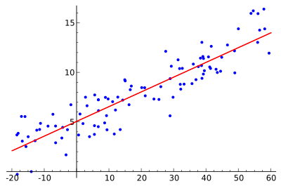
Visual understanding of multiple linear regression is a bit more complex and depends on the number of independent variables (p). If p = 1, this is just an instance of simple linear regression and the (x1, y) data points lie on a standard 2-D coordinate system (with an x and y-axis). Linear regression finds the line through the points that best “fits” the data.

Visual for p = 1 (https://en.wikipedia.org/wiki/Linear_regression)

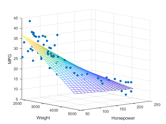
If p = 2, these (x1, x2, y) data points lie in a 3-D coordinate system (with x, y, and z axes) and multiple linear regression finds the plane that best fits the data points.

Visual for p = 2 (https://www.mathworks.com/help/stats/regress.html)

For greater numbers of independent variables, visual understanding is more abstract. For p independent variables, the data points (x1, x2, x3 …, xp, y) exist in a p + 1 -dimensional space. What really matters is that the linear model (which is p -dimensional) can be represented by the p + 1 coefficients β0, β1, …, βp so that y is approximated by the equation y = β0 + β1*x1 + β2*x2 + … + βp*xp.

Watch out!

There are two types of multiple linear regression: ordinary least squares (OLS) and generalized least squares (GLS). The main difference between the two is that OLS assumes there is not a strong correlation between any two independent variables. GLS deals with correlated independent variables by transforming the data and then using OLS to build the model with transformed data.

These procedures use the method of OLS. Therefore, to build a successful model you should first think through the relationships between your variables. It might not be a good idea to include bedrooms and accommodates as two separate independent variables, because it’s likely that number of bedrooms and number of guests accommodated have a strong positive correlation. On the other hand, there is no clear logical relationship between number of reviews and number of rooms. For a more quantitative analysis, pick independent variables so that each pair has a Pearson correlation coefficient near zero (see below).

Multiple LR in action

Alright, let’s go through a set of queries that build a multiple linear regression model in Neo4j.

Set up

Download and install the jar-file from the latest linear regression release. Run :play http://guides.neo4j.com/listings from the Neo4j browser and follow the import queries in order to create Will’s short term rental listing graph. Refer to my previous post for a more thorough guide to installing the linear regression procedures and importing the Austin rental data set.

Split training and testing data

Once you have the data set imported and procedures installed, we split the data set into a 75:25 (training:testing) sample. Let’s build from the final model from last time and again only consider listings with at least one review. Label 75% with :Train.

MATCH (list:Listing)-[:IN_NEIGHBORHOOD]->(:Neighborhood {neighborhood_id:'78704'}) 
WHERE exists(list.bedrooms) 
  AND exists(list.bathrooms)
  AND exists(list.price) 
  AND (:Review)-[:REVIEWS]->(list)
WITH regression.linear.split(collect(id(list)), 0.75) AS trainingIDs
MATCH (list:Listing) WHERE id(list) in trainingIDs 
SET list:Train

And add the :Test label to the remaining 25%.

MATCH (list:Listing)-[n:IN_NEIGHBORHOOD]->(hood:Neighborhood {neighborhood_id:'78704'})
WHERE exists(list.bedrooms) 
  AND exists(list.bathrooms)
  AND exists(list.price) 
  AND (:Review)-[:REVIEWS]->(list) 
  AND NOT list:Train 
SET list:Test

Quantify correlation

If you’d like to know the Pearson correlation between the independent variables, use the function regression.linear.correlation(List<Double> first, List<Double> second). One of the List<Double> inputs to this function contains aggregated “number of reviews” data from many listings, and each “number of reviews” is calculated by aggregating relationships from each listing. We cannot perform two levels of aggregation (collect(count(r))) in the same query. Therefore, we must perform two queries.

First store a num_reviews property on the data set listings.

MATCH (:Review)-[r:REVIEWS]->(list) 
WHERE list:Train OR list:Test
WITH list, count(r) AS num_reviews
SET list.num_reviews = num_reviews

Then collect (num_reviews, rooms) data from all listings and calculate correlation.

MATCH (list) 
WHERE list:Test OR list:Train
WITH collect(list.num_reviews) as reviews, 
     collect(list.bedrooms + list.bathrooms) as rooms
RETURN regression.linear.correlation(reviews, rooms)

Pearson’s correlation coefficients are in the range [-1, 1], with 0 meaning no correlation, 1 perfect positive correlation, and -1 perfect negative correlation. The number of reviews and number of rooms have a correlation -0.125, which indicates a very weak negative correlation. OLS is an acceptable method for this small correlation, so we can move forward with the model. Read more about interpreting correlation coefficients.

Initialize the model

We call the same create procedure but now our model framework is 'Multiple' instead of 'Simple' and the number of independent variables is 2 instead of 1.

CALL regression.linear.create(
          'mlr rental prices', 'Multiple', true, 2)

Add training data

Add known data in the same format as with simple linear regression. Just add another entry (number of reviews) to the list of independent variables.

MATCH (list:Train)
WHERE NOT list:Seen 
CALL regression.linear.add(
          'mlr rental prices', 
          [list.bedrooms + list.bathrooms, list.num_reviews], 
          list.price) 
SET list:Seen RETURN count(list)

Train the model

We must train the model so that line parameters (βi), coefficient of determination (R²), etc. are calculated before accepting testing data or making predictions. If you forget this step and then try to add testing data or make predictions, your model will automatically be trained first.

CALL regression.linear.train('mlr rental prices')

Note, you can still add more training data after calling the train procedure. You just need to make another call to train before testing the new model!

Add testing data

Analyze the model’s performance on unseen data. Remember that when you add test data, an additional parameter 'test' is required as input to the procedure regression.linear.add.

MATCH (list:Test) 
WHERE NOT list:Seen
CALL regression.linear.add(
          'mlr rental prices', 
          [list.bedrooms + list.bathrooms, list.num_reviews], 
          list.price, 
          'test') 
SET list:Seen 
RETURN count(list)

Test the model

Now that all the testing data is added, call the test procedure to calculate measurements (in testInfo below) that allow us to analyze the model’s performance.

CALL regression.linear.test('mlr rental prices')

You can also return information about the model at any time with a call to the info procedure.

CALL regression.linear.info('mlr rental prices') 

Let’s look at adjusted R². This value is similar to the R² we considered in my last post, but it is adjusted so that, as independent variables are added to the model, adjusted R² does not increase unless the model is improved more than it would by chance. Therefore, when comparing our multiple linear regression model (with two independent variables) to the prior model (with just one independent variable), adjusted R² is a better measurement of success.

We typically look for R² values greater than 0.6, but values closer to 1 indicate a better linear fit. Here, training adjusted R² = 0.517 and testing adjusted
R² = 0.556. Last time, our R² values were 0.500 and 0.559 for training and testing respectively. The model created with multiple linear regression performs a little bit better than the simple regression model from last time on training data, and about the same on testing data. Can you find better independent variables and improve my work?

A step back

At Neo4j, my colleagues and I are currently facing the question: Where do machine learning and artificial intelligence fit in with graph databases? There are several answers to this question, none of them the “right” answer. In my previous post, I demonstrated how a simple machine learning model can be built on data in the graph in order to avoid exporting to another software. In this post, another interesting aspect emerged: the ability to build models with data stored inherently in the graph’s structure. We were able to easily retrieve “number of reviews” data by counting the number of (:Review)-[:REVIEWS]->(:Listing) relationships on each listing. In this regard, graph databases increase the types of data we can easily access in order to build machine learning models.

Going forward, I would love to explore how machine learning models can more effectively utilize the graph structure of the data set to learn and make predictions.

Summary

Here’s a quick list of the tweaks you must make to use the regression.linear.* procedures for multiple linear regression:

• Specify model type “Multiple” during regression.linear.create
• Specify number of independent variables during regression.linear.create
• No regression.linear.remove method for testing or training data
• You cannot copy training data form one model to another with regression.linear.copy
• You should train the model with a call to regression.linear.train before testing, analyzing, or predicting
• Look at adjusted R² to more accurately compare models with different numbers of independent variables
• regression.linear.data returns the model’s parameters, not its byte[] serialization. Therefore, you cannot use regression.linear.load. (I would like to fix this)

This project is experimental, so I really appreciate any feedback. Checkout the procedure repository and reach out on LinkedIn or @ML_auren.

It’s time for me to move away from this linearly modeled world, and onto classifiers built with logistic regression. Stay tuned for a new set of procedures and a new data set!