Introduction to Classification Using K Nearest Neighbours
A Step by Step Approach to Build a KNN Classifier
As machine learning practitioners, we come across a wide array of machine learning algorithms that we may exert to build a particular predictive model. In this article, I will be focusing on one of the most sophisticated learning algorithm known as K Nearest Neighbour. This algorithm can be used for dealing with both regression and classification problems in ML.
In this article I will first try to give you an intuition of what the algorithm is, and how it makes predictions. Then I will try to break down certain important terms in affinity with this algorithm and finally by the end of this article, we will be designing our very own classifier using KNN algorithm.
Before starting this article, I would recommend you to take a look at my previous articles where I have discussed about various learning algorithms. Also if you like this article, do consider clapping for this article and make sure to follow me for more Machine Learning Recipes. The PDF copy of this article can be downloaded from here to continue your learning offline.
The Idea Behind the Algorithm
Suppose that you randomly select a ball from a bag full of metal balls that are either made of Gold or Carbon. In order to differentiate if either the ball is made of Gold or Carbon you can check its Colour, Electrical Conductivity, Boiling Point and Melting Point. These are referred to as the features. Using these features we can determine the class to which a ball belongs. This is analogous to how the KNN classification algorithm works.

The KNN algorithm is a simple, coherent yet versatile supervised learning algorithm that can be used to solve both classification and regression problems. It can essentially be considered as an algorithm that makes predictions based on the nature of other data points that are present close to it in the training dataset.
That is in simple terms, the classifier algorithm outputs the class to which the object is most likely to be assigned by calculating the similarity between the input sample and k training instances that are nearest to the input sample. It assumes that similar values exists in close proximity. KNN is often considered as a lazy learner as it doesn’t learn a discriminative function.
This algorithm is usually used when there is little or no information about the distribution of data. Also, the algorithm is non-parametric in nature which means that it does not make any underlying assumption about the data or in general its distribution pattern.

As a result the KNN algorithm requires no training time. However, whenever the algorithm is put into action, it needs to search the entire dataset to find the K nearest neighbours. This algorithm is mostly used for designing recommendation systems and performing analytical evaluation.
Under the Hood of KNN Classifier
Often the intricating part of solving a classification problem is finding the right algorithm to be used. Different algorithms work better with different types of data. KNN algorithm is generally used for datasets with fewer than 100K labeled non-textual data samples and are generally used when LinearSVC can not be put into action.
As mentioned previously, KNN is a supervised learning algorithm that can be used for handling both regression and classification problems. In this article we will be focussing on the KNN classifier.

The classifier takes the training data as an input and outputs the class to which an object is expected to belong to. This object is assigned to the class to which the majority of its neighbouring instances belong.
The K in KNN Classifier
K in KNN is a parameter that refers to the number of nearest neighbours to a particular data point that are to be included in the decision making process. This is the core deciding factor as the classifier output depends on the class to which the majority of these neighbouring points belongs.
Consider if the value of K is 5, then the algorithm will take into account the five nearest neighbouring data points for determining the class of the object. Choosing the right value of K is termed as Parameter Tuning. As the value of K increases the prediction curve becomes smoother.

By default the value of K is 5. There is no structure way to find the value of K, however the optimal value of K is the square root of the total number of samples that are present in the dataset. The value of K is generally taken as an odd value so as to avoid ties during decision making. An error plot or accuracy plot is generally used to find the most appropriate value of K.
Distance Metrics in KNN
For calculating distances KNN uses various different types of distance metrics. For the algorithm to work efficiently, we need to select the most appropriate distance metric. Some of these metrics are as mentioned below:
- Euclidean Distance: This is the default metric used by the sklearn KNN classifier. It is often referred to as L2 Norm. It calculates the ordinary straight line distance between two points in a Euclidean space.
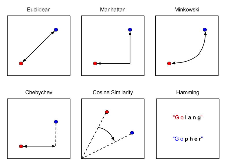
- Manhattan Distance: Often referred to as the city block metric, in this the distance between two points is the absolute differences of their Cartesian coordinates and is used in case of high dimensionality.
- Hamming Distance: This metric is used for comparing two binary data strings and is typically used with OneHotEncoding. It looks at the entire dataset and discovers when data points are similar or dissimilar.
Now that we have discussed the theoretical concepts of KNN classification algorithm, we will be applying our learning to build a classifier using K Nearest Neighbour algorithm. The code and other resources used for building this model can be found on my GitHub handle.
Step 1: Importing the Required Libraries and Datasets
The first step in building the classifier is to import all the necessary packages that will be used to build the classification model. To start with, we will be importing the Pandas, Numpy, Seaborn and Matplotlib package.
#Importing the Required Libraries and Loading the Dataset
import pandas as pd
import numpy as np
import seaborn as sns
import matplotlib.pyplot as plt%matplotlib inline
dataset = pd.read_csv("Iris.csv")
In this example we will be trying to classify an Iris flower species using various features such as its petal length, petal width, sepal length and sepal width. We need to be very careful while selecting the parameters for the model as KNN is highly sensitive to the parameters that are to be used.

Once all these libraries have been imported, the next step is to fetch the dataset. The data used for building this model can be downloaded from here. read_csv() function is used to load the dataset into the notebook. The dataset used for this model can be downloaded from here.
Step 2: Dividing the Data and Encoding the Labels
After loading the dataset, the next step is to split the data into features and labels. In machine learning, features are individual independent variables that are provided as an input to the system while labels are the attributes that we are trying to predict.
#Dividing Data Into Features and Labels
feature_columns = ['SepalLengthCm', 'SepalWidthCm', 'PetalLengthCm', 'PetalWidthCm']
X = dataset[feature_columns].values
y = dataset['Species'].values#Label Encoding
from sklearn.preprocessing import LabelEncoder
le = LabelEncoder()
y = le.fit_transform(y)

KNN classifiers do not accept string labels and thereby it is necessary to encode these labels before modelling the data. Label Encoders are used to transform these labels into numerical values.
Step 3: Visualising the Dataset
Visualising the dataset is an important step while building a classification model. It makes it easier to comprehend the data and look for some hidden patterns within the data. Python has a wide array of packages that can be used to visualise data.
#Visualizing Dataset using Pairplot
plt.figure()
sns.pairplot(dataset.drop("Id", axis=1), hue = "Species", size=3, markers=["o", "s", "D"])
plt.show()#Visualizing Dataset using Boxplot
plt.figure()
dataset.drop("Id", axis=1).boxplot(by="Species", figsize=(15, 10))
plt.show()
Matplotlib is the basis for static plotting in Python. Seaborn is one of the most popular library for plotting visually appealing graphs and is built on top of Matplotlib. Two such packages are Matplotlib and Seaborn that are used to plot data on various different types of charts.

The Matplotlib’s website contains multiple documentation, tutorials and a huge variety of examples, which makes its use a lot easier. Boxplot, Pairplot and Andrews Curves are few of the most widely used data visualization graphs that can be used to plot graphs to visualize classification problems.
Step 4: Splitting the Dataset and Fitting the Model
After selecting the desired parameters and visualizing the dataset, the next step is to import train_test_split from sklearn library which is used to split the dataset into training and testing data. We will by dividing the dataset into 80% training data and 20% testing data.
#Splitting the Data into Training and Testing Dataset
from sklearn.model_selection import train_test_split
X_train, X_test, y_train, y_test = train_test_split(X, y, test_size = 0.2, random_state = 0)#Fitting the Model and Making Predictions
from sklearn.neighbors import KNeighborsClassifier
from sklearn.metrics import confusion_matrix, accuracy_score
from sklearn.model_selection import cross_val_score

classifier = KNeighborsClassifier(n_neighbors=3)
classifier.fit(X_train, y_train)
y_pred = classifier.predict(X_test)
After this the KNeighborsClassifier is imported from the sklearn.neighbors package and the classifier is instantiated with the value of k set to 3. The classifier is then fit onto the dataset and predictions for the test set can be made using y_pred = classifier.predict(X_test).

Since in this example the features are in the same order of magnitude, no feature scaling is to be performed on the dataset. However it is recommended to normalize and scale the dataset before fitting a classifier.
Step 5: Evaluating the Predictions and Cross Validating
The simplest and the most commonly used technique to evaluate the prediction of a classification algorithm is by building the confusion matrix. Another method is to calculate the accuracy score of the model.
#Confusion Matrix
confusion_matrix = confusion_matrix(y_test, y_pred)
confusion_matrix#Calculating Model Accuracy
accuracy = accuracy_score(y_test, y_pred)*100
print('Accuracy of the model:' + str(round(accuracy, 2)) + ' %.')

#Performing 10 fold Cross Validation
k_list = list(range(1,50,2))
cv_scores = []
for k in k_list:
    knn = KNeighborsClassifier(n_neighbors=k)
    scores = cross_val_score(knn, X_train, y_train, cv=10, scoring='accuracy')
    cv_scores.append(scores.mean())#Finding Best K
best_k = k_list[MSE.index(min(MSE))]
print("The optimal number of neighbors is %d." % best_k)
After the output predictions have been evaluated, the next step is to perform multi-fold cross validation for parameter tuning. Herein, we are performing a ten fold cross validation to find the most optimal value of K.
Advantages of KNN Classifier
KNN classifier is one of the most sophisticated and widely used classification algorithm. Some of the features that make this algorithm so popular are as mentioned below:
- KNN does not make any underlying assumption about the data.
- It has a relatively higher accuracy than many classification algorithms.
- With the addition of more data points, the classifier constantly evolves and is capable of quickly adapting to the changes in input dataset.
- It gives the user the flexibility to choose the distance measure metric

Limitations of KNN Classifier
Though the classifier has multiple advantages, it also comes with certain crucial limitations. Some of these limitations are as mentioned below:
- KNN is very sensitive to outliers.
- As dataset grows, the classification becomes slower
- KNN is not capable of dealing with missing values.
- It is computationally expensive due to high storage requirements.
Summarizing What You Have Learned
To summarize what we have learned in this article, first we took a look into the idea behind the algorithm and its theoretical concepts. Then we discussed the parameter ‘K’ and learned how to find the most optimal value for K. After that we reviewed various Distance Measure metrics.

We then applied our learning to build a KNN classifier model to classify various plant species and then we propped up our learning by taking a glance on the advantages and limitations of the classification algorithm.
With that, we have reached the end of this article. I hope this article would have helped you get a hunch of how the KNN algorithm works. If you have any questions or if you believe I have made any mistake, feel free to contact me. Get in touch with me via: E-Mail or LinkedIn. Happy Learning!