Generative Adversarial Networks using Tensorflow
This post is a primer on Generative Adversarial Networks or simply called GANs.

Generative adversarial networks (GANs) are deep neural net architectures comprising of a set of two networks which compete against the other, hence the name “adversarial”. GANs were introduced in a paper by Ian Goodfellow and other researchers at the University of Montreal, including Yoshua Bengio, in 2014.
GANs are designed to mimic any distribution of data. That is, GANs can be taught to create worlds eerily similar to our own in any domain: images, music, speech, prose. To better understand what I mean by this, lets go through an example
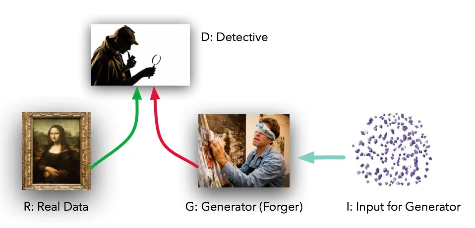
Let’s consider a scenario where a forger is trying to forge the famous portrait by Leonardo Da Vinci and a detective is trying to catch the forger’s paintings. Now, the detective has access to the real portrait and hence can compare the forger’s paintings to find even the slightest differences. So, in machine learning terms, the forger is called the “Generator” and generates fake data, and the detective is called the “Discriminator”, which is responsible for classifying the output of the generator as fake or real.
GANs are computationally expensive, in the sense that, they require high-powered GPU’s to produce good results. Below are some of the fake celebrity faces produced by GANs after training for several epochs on 8 Tesla V 100 GPU’s for 4 days!!
We will be using an less hardware intensive example. In this post, we will use the MNIST data set to play around with a simple GAN which will be made using Tensorflow’s layers API. Before, going into the code, I will discuss two problems that generally occur with the GANs:
- Discriminator overpowering Generator: Sometimes the discriminator begins to classify all generated examples as fake due to the slightest differences. So, to rectify this, we will make the output of the discriminator unscaled instead of sigmoid(which produces only zero or one).
- Mode Collapse: The generator discovers some potential weakness in the discriminator and exploits that weakness to continually produce a similar example regardless of variation in input.
So, finally, let’s get to the code!!
Firstly, we import the necessary libraries and read in the MNIST dataset from tensorflow.examples.tutorials.mnist .
Next, we will be creating two functions which respresent the two networks. Mind the second parameter “reuse”, I will explain it’s utility a little bit later.
Both the networks have two hidden layers and an output layer which are densely or fully connected layers.
Now, we create the placholders for our inputs. real_images are the actual images from MNIST and z is a 100 random pixels from the actual images. In order for the discriminator to classify it first has to know what the real images look like, so we have two calls to the discriminator function, the first two learn the actual images and the second two identify the fake images. reuse is set to true because when the same variables are used in two function calls the tensorflow computation graph gets an ambiguous signals and tends to throw value errors. Hence, we set the reuse parameter to True to avoid such errors.
Next, we define the loss function for our network. The labels_in parameter gives an target label for the loss function based on which it performs the calculations. The second argument for D_real_loss is tf.ones_like as we aim to produce true labels for all real images,but we add a bit of noise so as to address the problem of overpowering.
When we have two seperate networks interacting with each other we have to account for the variables in each networks scope. Hence, while defining the functions the tf.variable_scope was set. We will be using the Adam optimizer for this example. We set the batch_size and the number of epochs. Increasing the epochs lead to better results, so play around with it (preferably if you have access to GPU’s).
Finally, we initiate the session and use the next_batch() method from the tensorflow helper functions to train the networks. We, grab a random sample from the generated samples of the Generator and append it to the samples list.
Plotting the first value from the samples shows the generator performance after the first epoch. Comparing it to the last value from the samples shows how well the generator has performed.
The outputs look something like this:


These are very poor results, but as we are training our model merely on CPU the learning is quite weak. But as we can see the model is starting to generate pixels in a more concise way and we can kind of figure out that this digit is ‘3’.
GANs are meant to be trained on GPU’s, so try getting access to a GPU or simply try out google colab to get much better results.
All right, so this was a Generative Adversarial Network model built from scratch on Tensorflow. Click on the banner below to get the full code.
Till next time!!

