Thoughts and Theory
Gaussian Process Regression (GPR) is a remarkably powerful class of machine learning algorithms that, in contrast to many of today’s state-of-the-art machine learning models, relies on few parameters to make predictions. Because GPR is (almost) non-parametric, it can be applied effectively to solve a wide variety of supervised learning problems, even when little data is available. With state-of-the-art automatic differentiation frameworks such as PyTorch and TensorFlow, it’s easier than ever to learn and apply GPR to a multitude of complex supervised learning tasks.


In this article, we’ll discuss Gaussian Process Regression (GPR) from first principles, using mathematical concepts from Machine Learning, optimization, and Bayesian inference. We’ll start with Gaussian Processes, use this to formalize how predictions are made with GPR models, and then discuss two crucial ingredients for GPR models: covariance functions and hyperparameter optimization. Finally, we’ll build on our mathematical derivations below by discussing some intuitive ways to view GPR.
If you’d also like to see these ideas presented as an academic-style paper, please check out this link here. Let’s get started!
What is a Gaussian Process?
Before we talk about GPR, let’s first explore what a Gaussian Process is. A Gaussian Process falls under the class of random/stochastic processes, which define the realizations of random variables that evolve in space and/or time.
Rigorously, a Gaussian Process (GP) is a collection of random variables such that any subset of these variables is jointly Gaussian [1]. To represent a collection of d random **** variables as being jointly Gaussian, we can do so by expressing them as:
Where d is the number of random variables in the subset, μ is the vector of mean values, and Σ is the covariance matrix between these random variables. Written as a Gaussian density, a set of realizations for random variables x = (xi, …, xj) being jointly Gaussian implies:
One conceptualization of a GP is that it defines a distribution over functions [1]: Given a Gaussian Process, which is completely specified by a mean and covariance function, we can sample a function at the point x from the Gaussian Process according to:
Where f(·) is the function we sample from the GP, m(·) is a mean function, and k(·, ·) is a covariance function, which is a subclass of kernel functions. This is known as the function-space view of GPs [1].
Representing a dataset as a GP has a variety of applications in machine learning [1], signal processing [3], and probabilistic inference.
Now that we’ve introduced what a Gaussian Process is, we’re ready to start talking about how this probabilistic random process framework can be used for regression!
Gaussian Process Regression (GPR)
One application of Gaussian Processes is to perform regression via supervised learning, hence the name Gaussian Process Regression. This regression can be conceptualized as kernelized Bayesian linear regression, where the kernel parameterization is determined by the choice of covariance/kernel function, as well as the data used to make predictions [1]. This is known as the "weight-space view" of GPR [1].
Gaussian Process Regression can also be conceptualized in the aforementioned function-space view, in which the learner learns a distribution over functions [1] by learning mean and covariance functions of the realization of the GP at x, denoted by f(x).
The realization of a GP given by f(x) corresponds to a random variable. With these functions specified, f(x) can be sampled from the GP according to:
This is a formalization of sampling a random variable f(x) that depends on location x (for spatial applications; for time series applications, f(x) could depend on time t).
Estimates of the mean of f(x) are produced as a linear combination of observed target values y. The weighting coefficients used to produce these mean estimates are independent of the target values, placing Gaussian Process Regression models into the class of linear smoothers [1].
Given a training dataset consisting of N observations:
As well as a test dataset consisting of N’ points:
GPR predicts a posterior Gaussian distribution for targets over test points X∗ by computing the parameters of this Gaussian distribution given observed training data. We can think of this prediction as quite literally predicting a Gaussian distribution at each test point.
We will first consider the noise-free prediction case, and then use this to generalize to the case that models for noise in the observed target values y.
Please note the following definitions for the derivations below:
- m(·) represents a mean function
- K(· , ·) is a kernel/covariance function
- X is a (N, d) matrix of training features
- X∗ **** is a (N’, d) matrix of test points
- y is a (N, 1) vector of training targets
- f is a (N, 1) vector of realizations of the Gaussian Process on training features X
- f∗ is a (N’, 1) vector of realizations of the Gaussian Process on test points X∗
- Cov(·) is a covariance operator
- σ² is a positive hyperparameter denoting the covariance noise of the Gaussian Process.
We’re now ready to derive the predictions for GPR!
Noise-Free Prediction
Before we dive in, let’s recall our objective: Predict Gaussian distributions of targets f∗ at the test points X∗.
In the noise-free case, we have equality between the observed training targets y and the realized function values of the Gaussian Process f. Put another way, we observe the sampled functions of the Gaussian Process at points X directly.
Given the training and testing datasets defined above, the joint distribution of Gaussian process functions over the training and testing datasets (f and f∗, respectively) is given by [1]:
Where the covariance matrix on the right-hand side is a block matrix of kernel similarity matrices.
While the joint distribution gives some insight as to how f∗ relates to f, at this point no inference has been performed on the predictions f∗. Rather than this joint distribution, we are instead interested in the posterior distribution of the predicted GP realizations f∗ at the test points X∗. This is where the notion of Bayesian inference comes into play: We will condition our prior distributions over test points on our training data in order to improve our estimates of the Gaussian mean and variance parameters for our test points.
This posterior distribution can be computed by conditioning the predicted realizations of the Gaussian Process at the test points f∗ on the realized targets of the training dataset f. In addition to conditioning on f, we also condition on training inputs X and test inputs X∗.
We can therefore write the mean and covariance predictions at the test points X∗ as:
What do these estimates say?
- Predicted mean: This is estimated as a linear combination of the realizations of the Gaussian Process on the training set f. The coefficients of this linear combination are determined by the distance, in kernel space, between the test points X∗ and the training points X. Intuitively, this means that training samples closer in kernel space to X∗ have a stronger "say" in the predicted mean. These coefficients are also scaled by the inverse kernel similarity between the inputs in the training set X.
- Predicted covariance: This is estimated as the difference between the kernel distance between the test points X∗ minus a quadratic form of the inverse kernel distance of the training inputs X pre and post-multiplied by the kernel distance between the training and testing inputs.
In some applications, the mean function need not be zero, and can be written as a generalized m(·). In this case, with a non-zero mean function, the predicted mean and covariance estimates at the test points become:
Predicting in the Presence of Noise
In many applications of Gaussian Process Regression, it is common to model the training targets y to be noisy realizations of the Gaussian Process f [1], where noise is parameterized by a zero-mean Gaussian with positive noise covariance values given by σ².
This σ² is a hyperparameter that can be optimized (see the section below on hyperparameter optimization).
Using the predictive equations above along with our definition of noisy target values y, we can express the joint distribution over observed training targets y and predicted realizations of the Gaussian Process f∗ at test points X∗:
Using the same conditioning intuition and process as above, we can express the conditional distribution of predicted Gaussian Process realizations f∗ conditioned on observed training targets y as:
This is a lot to deconstruct, but the formulas for the predicted means and covariance are largely the same as before, simply with diagonal noise added to the inverse training kernel similarity term.
One practical consideration of adding covariance noise is that it can ensure the matrix in brackets remains positive semidefinite during GPR hyperparameter optimization, which in turn allows this matrix in brackets to be invertible.
The above derivations describe the exact analytical framework for how GPR makes predictions. However, some of the elements of these equations are still quite black-boxed, such as the kernel/covariance matrices and the covariance noise. In the sections below, we discuss these important elements of GPR.
Covariance Functions

Covariance functions are a crucial component of GPR models, since these functions weight the contributions of training points to predicted test targets according to the kernel distance between observed training points X and test points X∗. Recall from the previous section that one way to conceptualize GPR prediction is as a linear smoothing mechanism: The predicted means at test points X∗, in fact, can be expressed as:
Therefore, the predicted means are a linear combination of observed target values y, with output-independent weights determined by the kernel distance between the test points and the training point whose mean contribution is being taken into account.
Below are some example covariance functions that are frequently leveraged in GPR literature [1]:
- Squared Exponential (SE) / Radial Basis Function (RBF) Kernel with Automatic Relevance Determination (ARD) [4]. ARD enables learning separate lengthscales for each input dimension, and is therefore suitable for high-dimensional input spaces with variable scales and output sensitivity in each dimension. This covariance function is given by (where Θ is a diagonal matrix of lengthscales):
- Rational Quadratic (RQ) Kernel with ARD: The RQ kernel can be conceptualized as an infinite mixture of SE kernels, where the mixture weights are controlled by the positive hyperparameter α [1].
- Matérn Kernel with ARD: Under certain conditions, this kernel allows for perfect interpolation [1]. Note that ν is a hyperparameter that determines the degree of allowable discontinuity in the interpolation, K is a 2nd order Bessel function, and Γ(·) is the Gamma function.
Are Gaussian Process Regression Models Completely Non-Parametric?

Although Gaussian Process Regression models are considered to be non-parametric, their hyperparameters, such as lengthscales [1], significantly influence their predictive capabilities, and therefore should be optimized in order to maximize predictive out-of-sample performance. Fortunately, like many other supervised learning models, these hyperparameters can be optimized using gradient methods [1].
The objective for optimizing the hyperparameters of a GPR model is the marginal likelihood [1]. However, since this marginal likelihood has exponential terms, generally this optimization is performed by maximizing the marginal log-likelihood, in order to derive an analytic gradient update[1]. Since the marginal log-likelihood function is a strictly monotonic transformation of the marginal likelihood function, the set of hyperparameters that maximizes the marginal log-likelihood will also maximize the marginal likelihood.
The marginal log-likelihood, parameterized by a set of hyperparameters θ, is given by (when modeling noise in the observed targets):
As aforementioned, to optimize the hyperparameters of a GPR model, the derivatives of the marginal log-likelihood are computed with respect to θ [1]:
These derivatives are then used to update the hyperparameters of the GPR model using gradient ascent methods such as Adam [5]. This results in gradient updates of the form:
After the GPR’s hyperparameters have been optimized on the observed training dataset (X, y), the GPR model is ready to perform posterior inference on the test dataset X∗.
Review
So far, we’ve discussed: (i) How GPR models make predictions, (ii) Covariance functions for GPR, and the crucial role these functions play in determining similarity/distance between points, and (iii) How we can optimize the hyperparameters of GPR models to improve their out-of-sample performance.
Next, to strengthen our intuition, let’s discuss some other interpretations of GPR.
What Are Some Other Ways We Can Think About GPR?
Like other machine learning techniques and algorithms, there are many interpretations of Gaussian Process Regression (GPR). Here are a few that tie into what we discussed above. GPR is an algorithm that:
- Computes the joint multivariate Gaussian posterior distribution of a test set given a training set. This is formalized as sampling a function from a Gaussian Process.
- Interpolates points in d-dimensional input (feature) space into m-dimensional output (target) space. Under certain conditions, these (test) predicted interpolated points are linear combinations of existing (training) points!
- Predicts the mean and standard deviation into the future, given the past and present.
- Performs regression in a high-dimensional feature space parameterized by covariance functions (positive semidefinite kernels).
Let’s discuss each of these using intuition and by applying the mathematical derivations above.
1. Joint Multivariate Gaussian Posterior
Perhaps this is where the "Gaussian" in Gaussian Process Regression comes in. This machine learning technique models the data as being derived from a Gaussian Process. Recall that a Gaussian Process is a collection of N random variables that are considered jointly-Gaussian.
Where does "posterior" fit in here? Well, like other supervised machine learning models, GPR relies on having both training and testing data. The model is fit with training data, and the predictions, in the form of a posterior distribution (in this case, a Gaussian posterior distribution) are defined as a conditional distribution of predictions for the test set conditioned on the observations from the training set).
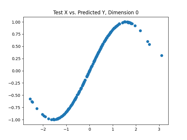
2. Interpolation


![Interpolation/kriging [2] was one of the first applications of Gaussian Process Regression [2]! Interpolation represents a prime use case of GPR, because we can interpolate the means and covariance of new points using existing points.](https://towardsdatascience.com/wp-content/uploads/2021/01/115Y9DQz84w87rTS2Z0KfZg.png)
GPR can also be used as a non-parametric interpolation method! This is also known as kriging in the spatial statistics field [2], and allows for interpolating both single and multi-dimensional outputs from single and multi-dimensional inputs.
Here, interpolation is performed using the same idea as above when computing predicted means: Interpolated points are estimated by taking combinations of the closest training points, and weighing them by their kernel distance ("similarity"). Points that are "closer" to the point in question contribute more of their output to the prediction of the new point than points that are "further away".
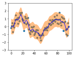
3. Predicting the Future Using the Past and Present
GPR is a common tool for time series forecasting because of its ability to capture temporal behaviors in a way that allows for the automatic measurement and weighting of how "close" two moments in time are.
Recall that since we predict a Gaussian posterior distribution, and since a Gaussian distribution is completely specified by its mean and variance parameters, then all that is needed to make predictions from this GPR is to predict the mean and variance going forward in time.
Predicting these quantities can actually be quite powerful – from this you can extract confidence intervals (mean +/ sqrt(variance)), as well as the predicted average/expected value of your quantities of interest over time.
4. Measuring "Closeness" In High-Dimensional Feature Space Using Covariance Functions
A final exciting interpretation of GPR is that it is effectively Bayesian Regression with a feature space composed of a possibly infinite-dimensional set of basis functions!
This result is a consequence of Mercer’s Theorem. A partial statement of the theorem is given below:
The functions φ(x) and its conjugate φ*(x’) are the eigenfunctions of the kernel (in our case, covariance) function ** k(x, ** x’). These eigenfunctions are special because integrating them over a measure, such as a probability density p(x) or Lebesgue measure [1], results in the eigenfunction itself, scaled by a number called the eigenvalue, denoted here by λ. We can think of this expression above as _a generalized Fourier Seri_es representation of our kernel [1]. Notice that this means we can have an infinite number of basis functions we can use to transform our inputs into features. This is similar in principle to the kernel trick.
Combining this result with the linear smoothing function result above, we can rewrite our expression for the latent predictions as a weighted sum of eigenvalue-eigenfunction combinations:
What is relevant about the result above? We have shown that the linear combinations of the outputs used to form the prediction are determined by the eigenfunctions and eigenvalues of the covariance function applied at the training and testing points. Aside from the choice of covariance function and covariance noise, predictions here are determined entirely from the data itself! This illustrates why Gaussian Process Regression is considered to be non-parametric.
Even if eigenfunction analysis isn’t really your cup of tea, there is an important takeaway to be had here: GPR transforms our standard Bayesian Regression setup into an infinite-dimensional feature space through the covariance function! Depending on the choice of covariance function, this can admit unlimited expressive power for our GPR model. This is part of what makes GPRs so powerful and versatile for a wide range of supervised machine learning tasks.
How Can I Learn More?
Below are just a few (very helpful) resources to get you started. This list is certainly not exhaustive:
- Gaussian Processes for Machine Learning [1]: A mathematically-rigorous textbook on Gaussian Processes. This book focuses a lot on the probabilistic and geometric theory behind GPR, such as kernels, covariance functions, measures, estimation, and Reproducing Kernel Hilbert Spaces (RKHSs).
- Kernel Cookbook: A great guidebook for the point in your GPR learning track in which you ask yourself: "What GPR covariance function should I use when?" This guide combines intuition with mathematical rigor.
- Automatic Relevance Determination (ARD): As introduced in the covariance functions section, ARD is particularly useful for GPR problems with variable feature scales and output sensitivity across input dimensions.
Wrap-Up And Review
In this article, we introduced Gaussian Processes (GPs) and Gaussian Process Regression (GPR) models, as well as some of their theoretical and intuitive underpinnings.
In our next article on GPR, I will go over some applications and implementation resources for GPR models.
To see more on reinforcement learning, computer vision, robotics, and machine learning, please follow me. Thank you for reading!
Acknowledgments
Thank you to CODECOGS for their extremely useful inline equation rendering tool, as well as to Carl Edward Rasmussen for open-sourcing the textbook Gaussian Processes for Machine Learning.
References
[1] Carl Edward Rasmussen and Christopher K. I. Williams. 2005. Gaussian Processes for Machine Learning (Adaptive Computation and Machine Learning). The MIT Press.
[2] Oliver, Margaret A., and Richard Webster. "Kriging: a method of interpolation for geographical information systems." International Journal of Geographical Information System 4.3 (1990): 313–332.
[3] Oppenheim, Alan V, and George C. Verghese. Signals, Systems & Inference. Harlow: Pearson, 2017. Print.
[4] Husmeier D. (1999) Automatic Relevance Determination (ARD). In: Neural Networks for Conditional Probability Estimation. Perspectives in Neural Computing. Springer, London. https://doi.org/10.1007/978-1-4471-0847-4_15
[5] Kingma, Diederik P., and Jimmy Ba. "Adam: A method for stochastic optimization." arXiv preprint arXiv:1412.6980 (2014).


