Gaining an intuitive understanding of Precision, Recall and Area Under Curve
A friendly approach to understanding precision and recall
In this post, we will first explain the notions of precision and recall. We will try not to just throw a formula at you, but will instead use a more visual approach. This way we hope to create a more intuitive understanding of both notions and provide a nice mnemonic-trick for never forgetting them again. We will conclude the post with the explanation of precision-recall curves and the meaning of area under the curve. The post is meant both for beginners and advanced machine learning practitioners, who want to refresh their understanding. At the end of the post, you should nevertheless have a clear understanding of what precision and recall are.
We will start our explanations with the case of a binary classification task. Binary means that each sample can belong only to two classes, e.g. dogs, cats. We will label samples belonging to the first class (cats) with 0’s and samples belonging to the second class (dogs) with 1’s.

In classification problems, neural networks are trained on labeled data. This means that each sample from the training, validation and test set was labeled by a human. The label assigned by a human is called ground truth.
In classification tasks the data is provided as pairs:
- input data
- ground truth label
Input data does not necessarily have to be images, it can also be text, sound, coordinates etc.
The input data is next fed to a neural network and we obtain a prediction to which class the sample belongs to. Please note, that precision-recall curves can only be calculated for types of neural networks (or more generally classifiers), which output a probability (also called confidence). In binary classification tasks, it is sufficient to output the probability that a sample belongs to class 1. Let us call this probability p. The probability of a sample belonging to class 0 is just:1 - p.
Hence if the neural network outputs p=0.99, it is quite confident, that the fed input data belongs to class 1, i.e. the input data is an image of a dog. If the networks outputs p=0.01 it is quite confident that the fed input data does NOT belong to class 1. This is equivalent that the fed input data belongs to class 0 with probability 1 - p = 0.99.
To get a concrete class prediction for a given sample, we usually threshold the output of the neural network using a threshold of 0.5. This means that a value above 0.5 is considered to belong to class 1, while a value below 0.5 is indicating class 0.
With all the definitions in hand, we can next define the notion of true positives, false positives, true negatives and false negatives.
True Positives, False Positives etc.
Now based on the output of the neural network we get the following four cases:
Case 1: True Positive
The input sample belongs to class 1 and the neural network correctly outputs a 1.

For historical reasons, this is called a True Positive. Remember: positive = 1.
Case 2: False Positive
The input sample belongs to class 0. The neural network however wrongly outputs a 1.

Case 3: True Negative
The input sample belongs to class 0 and the neural network correctly outputs a 0.

Again for historical reasons this is called a True Negative. Remember: negative = 0.
Case 4: False Negative
The input sample belongs to class 1. The neural network however wrongly outputs a 0.

We will denote the number of true positives in a dataset as TP, the number of false positives as FP and so on. Please get really familiar with the notions of TP, FP, TN and FN before continuing reading.
Next, we will define the notion of precision.
Precision
We have the following dataset consisting of 10 samples:

Please note that the chosen dataset is imbalanced, i.e. the dog class is underrepresented with only 3 instances, compared to the cat class with 7 instances. Imbalance of data is almost always encountered when working with real datasets. In contrast, toy datasets like MNIST of CIFAR-10 have an equal distribution of classes. Precision and recall are particularly useful as metrics to assess the performance of neural networks on imbalanced datasets.
We feed each of the above input data into a neural network and obtain a probability/confidence for each sample:

Next, we sort the table according to the predicted confidence. We color actual positive samples with green color and actual negative samples with red color. The same color scheme is applied for positive and negative predictions. We assume again a threshold of 0.5.

The positive predictions can be split up into a set of TP and a set of FP.
We define precision to be the following ratio:

Hence the precision measures how accurate your positive predictions are, i.e. which percentage of your positive predictions is correct. Please note that the sum TP+FP corresponds to the total number of samples predicted as positive by the classifier.
Memorizing the definition of precision is a difficult task, still remembering it in a few weeks is even more difficult. What helped me a lot, was instead to memorize the colorful table above. Just keep in mind that precision is the length of the arrow above the first row (Actual) divided by the length of the arrow below the second row (Predicted) and keeping in mind that green represents ones (or positives).
Please note that FN are not used in the definition of precision.
To gain more insight into the notion of precision, let us vary the threshold which defines whether a sample is classified as positive or negative.
If we lower the threshold to be 0.3, we get a precision of 0.375. Remember for a threshold of 0.5 the precision was 0.5.

If we lower the threshold even further to be 0.0, we get a precision of 0.3. Important: this corresponds to the ratio of dogs in our dataset, since out of 10 samples 3 belong to the class dog.
We observe that decreasing the threshold also decreases the precision.
Next we increase the threshold to be 0.7 and get a precision of 0.75.

Last but not least we increase the threshold to 0.9 and obtain a precision of 1.0. Please note that in this case, we don’t have any false positives. We get one false negative, which as discussed above, is not considered in the calculation of precision.

Gathering all results we get the following graph:

We see that precision is bounded between 0 and 1. It increases when the threshold is increased. We also note that precision can be made arbitrarily good, as long as the threshold is made large enough. Hence precision alone cannot be utilized to assess the performance of a classifier. We need a second metric: the recall.
Recall
We have the following dataset consisting of 10 samples:

Please note that for clarity of explanation we are using a different dataset than before. The dog class is now overrepresented with 7 instances, compared to the cat class with only 3 instances.
We feed each of the above input data into a neural network and obtain the following confidences:

Again we sort the table according to the obtained confidence values. We use the same color scheme as before and assume again a threshold of 0.5.

This time we split the actual positives into a set of TP and a set of FN and define the recall to be the following ratio:

Hence the recall measures how good you find all the actual positives, i.e. which percentage of actual positive samples was correctly classified. Please note that the sum TP+FN corresponds to the total number of the actual positive samples in the dataset.
For memorizing the definition of recall you can again use the colorful table above. Recall is the length of the arrow below the second row (Predicted) divided by length of the arrow above the first row (Actual) and keeping in mind that green represents ones (or positives).
To gain more insight into the notion of recall, let us again vary the threshold which defines whether a sample is classified as positive or negative.
If we lower the threshold to be 0.3, we get a recall of 1.0. Remember that for the threshold of 0.5, the recall was 0.714. In contrast to precision, recall seems to increase when the threshold is decreased.

Please note that in the case above we don’t have any false negatives. We get one false positive, which as discussed above, is not considered in the calculation of recall. If we lower the threshold even further to be 0.0, we still get a recall of 1.0. This is due to the fact that already for the threshold of 0.3, all actual positives were predicted as positives. We also note that recall can be made arbitrarily good, as long as the threshold is made small enough. This is opposite to the behavior of precision and the reason why the two metrics work together so well.
Next, we increase the threshold to be 0.7 and get a recall of 0.571.

Last but not least we increase the threshold to 0.9 and obtain a recall of 0.285.

Gathering all results we get the following graph:

We see that recall is bounded between 0 and 1. It decreases when the threshold is increased. We also note that recall can be made arbitrarily good, as long as the threshold is made small enough.
Next, we will combine precision and recall to obtain the precision-recall curve (PR-curve).
Precision-recall Curve
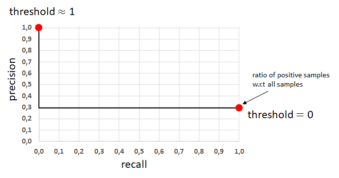
The precision-recall curve is obtained by plotting the precision on the y-axis and the recall on the x-axis for all values of the threshold between 0 and 1. A typical (idealized) precision-recall curve will look like the following graph:

We have seen that for very high thresholds (high means a little smaller than 1.0) the precision was very high and the recall was very low. This is represented by the red dot in the upper left corner of the graph.
For very low thresholds (a little larger than 0.0) we have shown, that the recall was almost 1.0 and the precision was identical to the ratio of positive samples in the dataset (!). This is shown in the graph by the red dot in the lower right corner.
The precision-recall curve of a perfect classifier looks as follows:

And the precision-recall curve of a very bad classifier (random classifier) will look like this:
With this knowledge you should now be able to judge whether an arbitrary precision-recall curve belongs to a good or a bad binary classifier. Please note that a correct interpretation of a precision-recall curve, however, requires that you also know the ratio of positive samples w.r.t. all samples.
1.1 Area Under the Precision-Recall Curve (PR-AUC)
Finally, we arrive at the definition of the metric PR-AUC. The general definition of PR-AUC is finding the area under the precision-recall curve:

as depicted in the graph below:
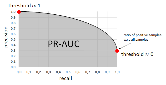
The PR-AUC hence summarizes the precision-recall curve as a single score and can be used to easily compare different binary neural networks models. Please note that the value of the PR-AUC for a perfect classifier amounts to 1.0. The value of PR-AUC for a random classifier is equal to the ratio of positive samples in a dataset w.r.t. all samples.
In our next post, we will show how to easily implement PR-AUC using Python.

