Create a Common-Sense Baseline First
When you set out to solve a data science problem, it is very tempting to dive in and start building models.
Don’t. Create a common-sense baseline first.

A common-sense baseline is how you would solve the problem if you didn’t know any data science. Assume you don’t know supervised learning, unsupervised learning, clustering, deep learning, whatever. Now ask yourself, how would I solve the problem?
Experienced practitioners do this routinely.
They first think about the data and the problem a bit, develop some intuition about what makes a solution good, and think about what to avoid. They talk to business end-users who may have been solving the problem manually.
They will tell you that common-sense baselines are not just simple to implement, but often hard to beat. And even when data science models beat these baselines, they do so by slim margins.

We will look at three examples, starting with a problem from direct marketing.
You work for an apparel retailer and have a customer database that has information on every customer who has bought something from you in the past year. You know what they bought, what they paid for it, and some demographic information as well.
You want to send out a mail piece advertising your latest line of Spring apparel and you have enough budget to mail up to 100,000 customers from the database.
Which 100,000 customers should you pick?
You are probably itching to create a training and test dataset and learn some supervised learning models. Perhaps Random Forests or Gradient Boosting. Or even Deep Learning.
These are all powerful models and they should be in your toolkit. But first, ask yourself this question: “If none of these methods existed and I had to live by my wits, how would I pick the best 100,000 customers?”.
Common-sense suggests that you should pick the most loyal customers in the database. After all, if anyone will find the mailer of interest, those customers will*.
And how would you measure loyalty? Intuitively, a loyal customer likely shops a lot and spends a lot. So you could calculate what each customer spent in the past year and how many times they shopped with you.
If you do this and look at the data, you will see that it captures loyalty quite well. But you’d also notice that it picks customers who were loyal in the first half of the year but who seemed to have fallen off the face of the earth in the second half.
You can fix this by seeing how recently the customer shopped with you. A customer who shopped with you yesterday is more valuable to you than a customer who shopped 11 months ago, if their spending and shopping frequency is otherwise similar.
To summarize, for each customer, you can calculate
- What they spent with you in the past 12 months
- Number of transactions in the past 12 months
- Number of weeks since the last transaction
You can decile the customer file based on these 3 metrics and sort the customer list accordingly.

Pick the top 100,000 customers.
Congratulations! You have just discovered the venerable Recency-Frequency-Monetary (RFM) heuristic, a tried-and-true workhorse of Direct Marketing.
In case you are wondering what’s more important as you go down the decile list — R, F or M — , R has been found to be the most important.
The RFM approach is easy to create, easy to explain and easy to use. Best of all, it is surprisingly effective. And experienced Direct Marketing practitioners will tell you that even when more sophisticated methods beat RFM, the gap between them will be much smaller than you think and will make you wonder if the complex stuff is worth the effort.
Next, an example from the product recommendations area.
The retailer you work for has an e-commerce site and you have been asked to build a product recommendation zone that will be displayed on the home page.

It needs to be personalized — if the visitor has been to your site before, you need to use whatever you have learned about them to recommend products that are tailored to their interests.
Entire books (example, example) have been written on this topic and GitHub repos (example, example) stand ready to serve you. Should you dive in and do matrix factorization?
You probably should at some point but not as the very first thing. You should create a common-sense baseline first.
What’s the simplest, relevant thing you can show visitors?
Top selling products!
Sure, they are not personalized. But top-selling products become top sellers because enough visitors buy them, so in that sense, chances are that at least some reasonable fraction of visitors will find them relevant even though they weren’t specifically chosen for them.
Moreover, you need to have top sellers ready anyway since you need something to show first-time visitors for whom you have no data.
Selecting top-sellers is simple. Decide on a time window (last 24 hours, last 7 days, ….), decide on a metric ( revenue, views, ….), decide how often to recalculate (hourly, daily, ….), write the query and stick it inside some automation.
And you can tweak this baseline in simple ways to make it a bit personalized. For example, if you remember the categories of the products viewed by the visitor in a previous visit, you can simply select top selling products from those particular categories (rather than from across all categories) and show them in the recommendation zone. A visitor who browsed the Women’s category in her previous visit may be shown top sellers from Women’s in the current visit.
To be clear, the ‘tweak’ described above will involve development work, since you need to ‘remember’ information across visits. But this will need to be done anyway if you are planning to build and deliver model-based personalized recommendations down the road.
Our final example is from retail price optimization.
As an apparel retailer, you sell seasonal merchandise — e.g. sweaters — that need to cleared out from the stores at the end of every season to make room for next season’s products. It is standard practice in the industry to mark down the price of these seasonal products to motivate shoppers to buy them.

If you discount too little, you will have merchandise left over at the end of the season that you will have to dispose of at salvage prices. If you discount too much, you will sell out of the product but lose the opportunity to make more money.
In the industry, this balancing act is called clearance optimization or markdown optimization.
There’s a ton of literature on how to model and solve this problem using data science techniques (for example, see Chapter 25 in the Oxford Handbook of Pricing Management. Disclosure: I wrote it).
But let’s first think about how to create a common-sense baseline.
Imagine that you have 100 units of a sweater on hand and 4 weeks left in the current season. You can change prices once a week, so you have four chances to do something.
Should you cut the price this week?
Well, for starters, it depends on how many units you think you can sell in the next 4 weeks if you left the price unchanged.
How can we get a sense for this? The simplest thing we can do is to look at how many units sold last week.
Assume we sold 15 units. If the next 4 weeks are similar to the last week, we will sell 60 units and end the season with 40 units still unsold.
Not good. Clearly a price cut is in order.
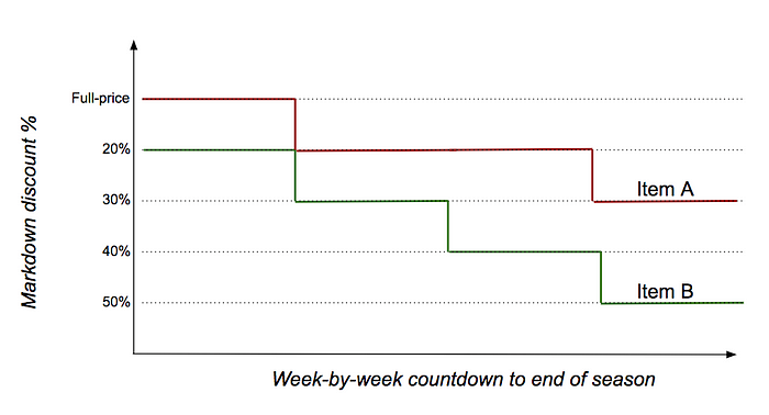
Retailers sometimes use discount ladders — 20% off, 30% off, 40% off, … — and the price cuts have to be on the ladder. The simplest thing to do is to step on to the first rung of the ladder i.e., discount the price by 20% for the next week.
Fast forward one week. Let’s say you sold 20 units last week. You now have 80 units remaining and 3 weeks to go. If the same rate-of-sale (e.g. 20 units per week) is maintained for the next three weeks, you will sell 60 units in the remaining 3 weeks, and will have 20 units left unsold at the end of the season. So, you step down another rung on the ladder and increase the discount to 30% off.
You get the idea. Repeat each week till you reach the end of the season.
Different products may follow different discount paths depending on how their selling rates respond to discounts. In the example below, Item B required more discount stimulation than Item A.

This common-sense baseline can be implemented with very simple if-then logic. And like the personalized recommendations example above, it can be tweaked (e.g., instead of using just the last week’s sales units as the ‘forecast’ for the future weeks, average the last few weeks instead).
With the baseline in place, you can now go forth and throw all the data science firepower you can at this problem. But compare whatever you do with the results of the common-sense baseline to accurately gauge the return-on-effort.
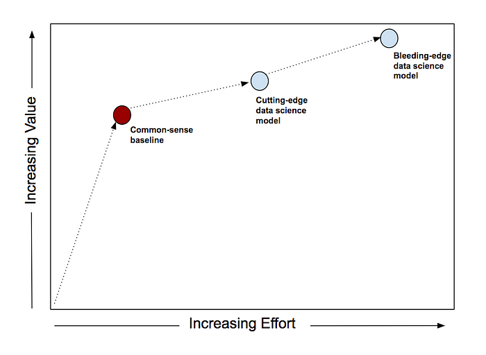
In many problem areas, the venerable 80–20 principle is alive and well. And a common-sense baseline often gets you to the 80% mark very fast.
As you throw more and more data science at the problem, you will see more value but at a diminishing rate. Now, depending on your specific situation, you may well decide to go with a sophisticated approach to extract those last chunks of value. But you should do so with a clear idea of the incremental costs and benefits.
Ultimately, a common-sense baseline protects you against a danger famously described by Richard Feynman.
The first principle is that you must not fool yourself — and you are the easiest person to fool.
Building data science models can be very enjoyable and it is easy to be lulled into thinking that your sophisticated, lovingly-created-and-tuned model is better (from a cost/benefit perspective) than it really is.
Common-sense baselines deliver value quickly and protect you from yourself. Make them a habit.
*There’s a different way to think about this problem — Uplift Modeling — which considers the incremental effect of sending a customer a mailer.


