
As mentioned in my article about Summarizing text, I have a collection of news articles spanning the last decade. After summarizing these articles, the next challenge I faced was finding related articles. If I have one article, how do I find articles related to this article? Immediately resulting in the question what is a related article?
After some initial research TF-IDF is chosen as algorithm. It is an old algorithm with limited complexity, so it possible to create an implementation and learn from this how finding similar articles work. As often, there are better implementations available, e.g. in scikit-learn, but I prefer building my own for learning purposes. Be ware, the full implementation will take some time.
The TF-IDF algorithm
So, what is TF-IDF? When we breakdown the abbreviation, it says Term Frequency – Inverse Document Frequency, a mouthful. Term Frequency refers to the relative number of times a specific term (word) occurs in a text:

The TF of term t in document d is equal to the frequency term t appears in document d, divided by the sum of frequencies for all terms t’ in document d. Example:
'The green man is walking around the green house'
TF(man) = 1 / 9 = 0.11
TF(green) = 2 / 9 = 0.22
This is a measure of how important a word is in a document, corrected for the length of the document.
The IDF is a measure for the importance of the word in the whole corpus (the set of all documents analysed). The idea is that if a word occurs in a lot of documents, it does not add a lot of information. The standard function is
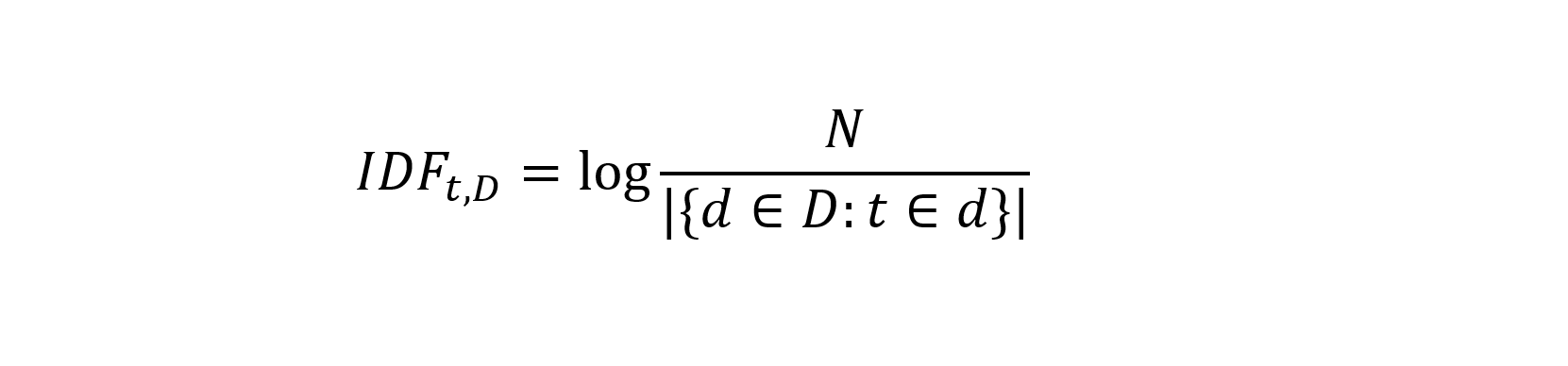
The IDF is calculate by dividing the number of documents (N) by the total number of documents a term occurs in and taking the logarithmic value of this. If a term occurs 10 times in 10.000 documents, the IDF equals 3. A term occurring 100 times in the same set of documents will have an IDF value of 2. When a term occurs in all documents, the IDF value equals 0.0. The logarithmic value is used to reduce the large range of values the IDF can have.
Finally, the TF-IDF value of a term, equals TF multiplied by IDF:

The formulas above are the standard formulas for TF and IDF. More variants can be found on the wikipedia page of TF-IDF.
The TF-IDF value is calculated for each word in the corpus for all documents, including the documents the number of occurrences of the term is 0. AS an example, the following two sentences
0: 'the man walked around the green house',
1: 'the children sat around the fire'
result in the following TF-IDF values:

For all unique words the TF-IDF value is calculated for each sentence. This value is 0.0 when
- a specific word does not occur in a sentence (e.g. ‘green’ in the second sentence) due to the TF being 0.0
- a specific word occurs in all sentences, e.g. ‘around’ due to the fact that the logarithmic value of 1 equals 0.0. In this case, the TF-IDF value is 0.0 for all sentences
Calculating distance
Now that the TF-IDF values are calculated, the distance between two documents can be determined by calculating the cosine similarity between these values. This is done by using the TF-IDF values per word, one row in the dataframe above, as a vector.
The cosine distance is the difference in angle between the lines from the origin to two points in a N-dimensional space. It is relative simple to visualize in two dimensions. The example above is in 9 dimensions and surpasses my imagination. In two dimensions:

The cosine difference can be calculated using the Eucledian dot product formula:

It is the dot-product of two vectors divided by the multiplication of the vector lengths. When two vectors are parallel the cosine difference is 1.0, and when they are orthogonal the value is 0.0.
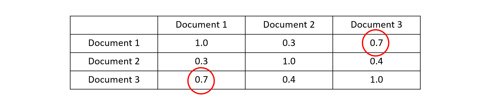
This function needs to be applied to all combination of documents in the corpus. The difference from A to B is equal to the difference from B to A and the difference from A to A is 1.0. The table below shows that the matrix with distances is mirrored across the diagonal:
After all this math it is time to start the implementation!
Implementing TF-IDF
Well done, you have survived the theoretical background! But now the question is how to implement this functionality. The goal is to calculate the distance between several documents. Working backwards, we need the TF-IDF to calculate the dstances and we need the TF and IDF to calculate the TF-IDF.
Calculating TF and IDF require some processing of documents. We need the occurances per word per document and the total number of words in a document for the TF and the number of documents each word occurs in and the numer of documents for the IDF. These require same common document parsing, so a pre processing step is added:
class DocumentDistance:
    distancespre = {}

    def add_documents(self, docs: typing.List[str],
                      ) -> None:
        """
        Calculate the distance between the documents
        :param documents: list of documents
        :return: None
        """
        word_occ_per_doc, doc_lens, doc_per_word = self.pre_proces_data(docs)

        # Calculate TF values
        tfs = []
        for i in range(len(word_occ_per_doc)):
            tfs.append(self.compute_tf(word_occ_per_doc[i], doc_lens[i]))

        # Calculate IDF values
        idfs = self.compute_idf(doc_per_word, len(docs))

        # Calculate TF-IDF values
        tfidfs = []
        for i in range(len(tfs)):
            tfidfs.append(self.compute_tfidf(tfs[i], idfs))

        # Calculate distances
        self.calculate_distances(tfidfs)
A class is defined that will store the distances between all documents as a two dimensional array. This array will be filled from the calculate_distances method. But first, we will create the pre_process_data method that will parse all documents from a list and return the word occurences per document, the document lengths, and the number of documents each word occurs in:
  from Nltk import word_tokenize

  class DocumentDistance:

      ...

      def pre_proces_data(self,
                        documents: typing.List[str]
                        ) -> (typing.Dict[int, typing.Dict[str, int]],
                             typing.Dict[int, int],
                             typing.Dict[str, int]):
        """
        Pre proces the documents
        Translate a dictionary of ID's and sentences to two dictionaries:
        - bag_of_words: dictionary with IDs and a list with the words in the text
        - word_occurences: dictionary with IDs and per document word counts
        :param documents:
        :return: dictionary with word count per document, dictionary with sentence lengths
        """
        # 1. Tokenize sentences and determine the complete set of unique words
        bag_of_words = []
        unique_words = set()
        for doc in documents:
            doc = self.clean_text(doc)
            words = word_tokenize(doc)
            words = self.clean_word_list(words)
            bag_of_words.append(words)
            unique_words = unique_words.union(set(words))
        # 2. Determine word occurences in each sentence for all words
        word_occurences = []
        sentence_lengths = []
        for words in bag_of_words:
            now = dict.fromkeys(unique_words, 0)
            for word in words:
                now[word] += 1
            word_occurences.append(now)
            sentence_lengths.append(len(words))

        # 3. Count documents per word
        doc_count_per_word = dict.fromkeys(word_occurences[0], 0)
        # Travese all documents and words
        # If a word is present in a document, the doc_count_per_word value of
        # the word is increased
        for document in word_occurences():
            for word, val in document.items():
                if val > 0:
                    doc_count_per_word[word] += 1

        return word_occurences, sentence_lengths, doc_count_per_word
The first part splits a document into words by tokenizing the documents with the help of word_tokenize, part of the NLTK package. Before tokenizing some document cleaning takes place, like transforming the document to lowercase (discussed later on). The word list is cleaned in the clean_word_list method, which is empty for now. The list with tokens per document is stored in the bag_of_words variable, which is a list with an entry per document, containing a list of tokens. During this loop, a set of all unique words is created. This set unique_words contains all uniqee words occurring in the corpus.
Step 2 determines for all document the number of occurrences for all unique words. For each document (the loop over bag of words) a dictionary is created with the value 0 (zero) for all unique words (dict.fromkeys(...)). Then the code iterates over all words in the document and increases the dictionary value with 1 (one). This dictionary is added to word_occurences to create a list of dictionaries for all documents with the word count and the document length is stored in sentence_lengths.
The last step, step 3, counts per word the number of documents it occurs in. First a list doc_count_per word with 0 (zero) occurrences per unique word is created. A word is present in a document when the word count of this specific word in a document is greater than zero.
The result of the preprocessing is:
Documents:
'the man walked around the green house'
'the children sat around the fire'

word_occurences:
{
 0: {'green': 1, 'fire': 0, 'house': 1, 'sat': 0, 'around': 1, 'man': 1,
     'the': 2, 'children': 0, 'walked': 1},
 1: {'green': 0, 'fire': 1, 'house': 0, 'sat': 1, 'around': 1, 'man': 0,
     'the': 2, 'children': 1, 'walked': 0}
}

sentence_lengths:
[7, 6]

doc_count_per_word:
{'around': 2, 'green': 1, 'house': 1, 'walked': 1, 'sat': 1,
 'children': 1, 'man': 1, 'fire': 1, 'the': 2}
With these data sets the TF and IDF can be calculated relatively straight forward:
    def compute_tf(self,
                   wordcount: typing.Dict[str, int],
                   words: typing.List[str]
                   ) -> typing.Dict[str, float]:
        """
        Calculates the Term Frequency (TF)
        :param wordcount: dictionary with mapping from word to count
        :param words: list of words in the sentence
        :return: dictionary mapping word to its frequency
        """
        tf_dict = {}
        sentencelength = len(wordcount)
        for word, count in wordcount.items():
            tf_dict[word] = float(count) / sentencelength
        return tf_dict

    def compute_idf(self,
                    doc_count_per_word: typing.List[typing.Dict[str, int]],
                    no_documents: int
                    ) -> typing.Dict[str, int]:
        """
        Calculates the inverse data frequency (IDF)
        :param doc_count_per_word: dictionary with all documents. A document is a dictionary of TF
        :param no_documents: number of documents
        :return: IDF value for all words
        """
        idf_dict = {}
        for word, val in doc_count_per_word.items():
            idf_dict[word] = math.log(float(no_documents) / val)
        return idf_dict

     def compute_tfidf(self,
                       tfs: typing.Dict[str, float],
                       idfs: typing.Dict[str, float]
                       ) -> typing.Dict[str, float]:
        """
        Calculte the TF-IDF score for all words for a document
        :param tfs: TFS value per word
        :param idfs: Dictionary with the IDF value for all words
        :return: TF-IDF values for all words
        """
        tfidf = {}
        for word, val in tfs.items():
            tfidf[word] = val * idfs[word]
        return tfidf
The compute_tf method is called per document. The TF values per word are calculated by dividing the number of occurrences by the length of the sentence (The calculation result is forced ti a float type).
The compute_idf is called with the documents count for each word and the total number of documents. The discussed formula is applied to these values.
And finally the TF-IDF values per word per sentence are calculated by multiplying the TF value with the corresponding IDF value.
tfs:
[{'sat': 0.00, 'green': 0.14, 'walked': 0.14, 'the': 0.28,
  'around': 0.14, 'children': 0.00, 'fire': 0.00, 'man': 0.14,
  'house': 0.14},
 {'sat': 0.16, 'green': 0.00, 'walked': 0.00, 'the': 0.33,
  'around': 0.16, 'children': 0.16, 'fire': 0.16, 'man': 0.00,
  'house': 0.00}]

idfs:
{'sat': 0.69, 'green': 0.69, 'walked': 0.69, 'the': 0.00,
 'around': 0.00, 'children': 0.69, 'fire': 0.69, 'man': 0.69,
 'house': 0.69}

tfidfs:
[{'sat': 0.00, 'green': 0.09, 'walked': 0.09, 'the': 0.00,
  'around': 0.00, 'children': 0.00, 'fire': 0.00, 'man': 0.09,
  'house': 0.09},
 {'sat': 0.11, 'green': 0.00, 'walked': 0.00, 'the': 0.00,
  'around': 0.00, 'children': 0.11, 'fire': 0.11, 'man': 0.00,
  'house': 0.0}
]
Now that we have the TF-IDFS values, it is possible to calculate the distance between the different documents:
Python">    def normalize(self,
                  vector: typing.Dict[str, float]
                  ) -> float:
        """
        Normalize the dictionary entries (first level)
        :param tfidfs: dictiory of dictionarys
        :return: dictionary with normalized values
        """
        sumsq = 0
        for i in range(len(vector)):
            sumsq += pow(vector[i], 2)
        return math.sqrt(sumsq)

def calculate_distances(self,
                        tfidfs: typing.List[typing.Dict[str, float]]
                        ) -> None:
    """
    Calculate the distances between all elements in tfidfs
    :param tfidfs: The dictionary of dictionaries
    :return: None
    """
    vectors = []
    # Extract arrays of numbers
    for tfidf in tfidfs:
        vectors.append(list(tfidf.values()))

    self.distances = [[0.0] * len(vectors) for _ in range(len(vectors))]
    for key_1 in range(len(vectors)):
        for key_2 in range(len(vectors)):
            distance = np.dot(vectors[key_1], vectors[key_2]) /
                       (self.normalize(vectors[key_1])* self.normalize(vectors[key_2]))
            self.distances[key_1][key_2] = distance
As described in the first part of this article, the cosine distance between two vectors is calculated by dividing the dot product of the vectors by the product of the normalized vectors.
To calculate the dot product, the dot method from the numpy library is used. The dot product is calculated by summarizing pairwise multiplied values:

The normalized value of a vector equals the length of the straight line between the origin and the point identified by the vector. This equals the square root of the sum of the squares of each dimension:

The normalization of a vector is implemented in the normalize() method. The distance between all combination of vectors is calculated in the calculate_distances() method. All distances are stored in the distances attribute of the class. Before calculating the distances, this variable is initialized as a _N_xN matrix of 0.0 values.
An example:
Sentences:
'the man walked around the green house'
'the children sat around the fire'
'a man set a green house on fire'

Distances:
[1.00, 0.28, 0.11]
[0.28, 1.00, 0.03]
[0.11, 0.03, 1.00]
Notice that the distance is minimal with value 1.0 and maximal with 0.0. Since both sentences have no words in common, their distance is 0.0. The distance between a sentence and itself is 1.0.
Performance improvements
With a corpus of three documents, each consisting of a small sentence, the distances are calculated fast. This time increases fast when the documents become articles and the number increases to the hundreds. The graph below show the number of unique words as function of the number of news articles.

When 1.000 articles are processed, the number of unique words increases to almost 15.000. This means that each vector, describing a document has 15.000 entries. One dot multiplication takes 225 million multiplications and 225 million additions. Per vector. Normalizing one vector is also 225 million multiplications (calculating the square), 225 million additions and one square root. So one distance calculation between two vectors is 775 milion multiplications, 775 million additions, 1 square roott, one division and one addition. And all this 1 million times to fill the whole array of distances. One can imagine this takes some time…
So how can we reduce the amount of work? The golden rule is to do as little as little time as possible. So let’s see what we can do to optimize.
Distance calculation
It was already mentioned in the first part, that the matrix of distances contains duplicate values. The distance from A to B is equal from the distance from B to A. We only have to calculate it once and add it in two places to the matrix.
Secondly, the diagonal of the matrix is 1.0 since the distance between A and A is always 1.0. No calculations required here. These two steps will half the number of distances calculated.
And thirdly, all vectors are normalized for each calculation. This is superfluous. We can pre-calculate all normalizations and store it for re-use in array. This will reduce the distance calculation by 2/3, only the dot calculation needs to be calculated for every combination of vectors.
These there improvements reduce the required time by 85%!
def normalize(self,
              tfidfs: typing.List[typing.Dict[str, float]]
              ) -> typing.Dict[int, float]:
    """
    Normalize the dictionary entries (first level)
    :param tfidfs: dictiory of dictionarys
    :return: dictionary with normalized values
    """
    norms = []
    for i in range(len(tfidfs)):
        vals = list(tfidfs[i].values())
        sumsq = 0
        for i in range(len(vals)):
            sumsq += pow(vals[i], 2)
        norms.append(math.sqrt(sumsq))
    return norms

def calculate_distances(self,
                        tfidfs: typing.List[typing.Dict[str, float]]
                        ) -> None:
    """
    Calculate the distances between all elements in tfidfs
    :param tfidfs: The dictionary of dictionaries
    :return: None
    """
    norms = self.normalize(tfidfs)
    vectors = []
    # Extract arrays of numbers
    for tfidf in tfidfs:
        vectors.append(list(tfidf.values()))

    self.distances = [[1.0] * len(vectors) for _ in range(len(vectors))]
    for key_1 in range(len(vectors)):
        for key_2 in range(key_1 + 1, len(vectors)):
            distance = np.dot(vectors[key_1], vectors[key_2]) / (norms[key_1] * norms[key_2])
            self.distances[key_1][key_2] = distance
            self.distances[key_2][key_1] = distance
Some small changes to the code lead to an 85% reduction in calculation time. But there is more possible
Reducing vector size
The distance calculation was the most expensive part of the code. The changes above have reduced the calculation time significantly. But there is another aspect greatly impacting the performance, and that is the size of the document vectors. With the 1.000 articles, each document vector is 15.000 elements. If we are able to remove this vector size,the calculation times will benefit.
So what can we do to reduce the vector size? How do we find the elements without impact that can be removed? Looking at the IDF function, it shows that stop words have no impact on the distance calculation. They appear in every document and thus the IDF value and TF-IDF will be 0.0 in all vectors. Multiplying all these zeros still takes time, so the first step is to remove the stopwords from the list of unique words.
Stopwords per language are available in the NLTK toolkit. The toolkit provides the list of stopwords and these can be filtered from the unique words.
Second, a word that occurs in only one document is always multiplied by a zero for all other documents. We can safely remove this word from the vectors.
Finally, the last step is to use stemming. The wordlist will contain words like ‘house’ and ‘houses’. By combing these to house, same meaning afterall, we can reduce the wordlist even more ánd increase the quality of the overall algorithm. It will no longer see ‘house’ and ‘houses’ as different words but as one. NLTK provides several stemmers, supporting multiple languages of which the SnowballStemmer is used.
Stemming also reduces all verbs to there base. Words as ‘like’, ‘liking’, ‘liked’, etc will all be reduced to there stem ‘like’.
The method reduce_word_list was already introduced (but empty) so now we can use it to apply these rules:
from nltk.stem.snowball import SnowballStemmer
from nltk.corpus import stopwords

stop_words = set(stopwords.words("dutch"))
stemmer = SnowballStemmer("dutch")

def clean_word_list(self, words: typing.List[str]) -> typing.List[str]:
    """
    Clean a worlist
    :param words: Original wordlist
    :return: Cleaned wordlist
    """
    words = [x for x in words if x not in self.stop_words and
                                 len(x) > 2 and not x.isnumeric()]
    words = [self.stemmer.stem(plural) for plural in words]
    return list(set(words))
The second rule, remove words only present in one document, is applied in an altered version of the pre processing function by adding a fourth step after the third:
        # 4. Drop words appearing in one or all document
        words_to_drop = []
        no_docs = int(len(documents) * .90)
        for word, cnt in doc_count_per_word.items():
            if cnt == 1 or cnt > no_docs:
                words_to_drop.append(word)
        for word in words_to_drop:
            doc_count_per_word.pop(word)
            for sent in word_occurences:
                sent.pop(word)
The first loop collects the words occurring once or always are collected. It is not possible to modify the word lists during this loop, as it will alter the collection used for iterating. A second step is needed to remove (pop) the superfluous words from the document counter and each document. It is a relative expensive operation, but the reduction in vector size is worth it.
Curious to the effect of all these vector reduction steps? Lets see:

The blue line is the original number of unique words. The grey line is the reduced number of words. So at 1.000 articles the number of words is reduced from 15.000 to 5.000. Each vector multiplication is reduced by 66%.
The code is profiled with cProfile and the results are visualized with snake_viz. The execution time of the original code:

Adding documents takes 31.2 seconds, of which 29.6 seconds are spent calculating distances and 0.4 seconds pre processing data.
29.6 calculate_distance(...)
 0.6 compute_tf(...)
 0.4 pre_proces_data(...)
 0.4 compute_tfidf(...)
 0.1 compute_idf(...)
The execution time of the optimized version:

The time it takes to add the document now takes 5.39 seconds (was 31.2) of which 4.32 seconds (was 29.6) are spent calculating distances and 0.9 seconds processing data (was 0.4).
So the pre-processing takes double time, adding 0.5 seconds to the execution time, but the distance calculations only take 14% of the original time. The extra time pre-processing is earns itself back easily.
 4.2 calculate_distance(...)
 0.9 pre_proces_data(...)
 0.1 compute_tf(...)
 0.0 compute_tfidf(...)
 0.0 compute_idf(...)
Happy?
So, happy with the results? To be honest, no. I really liked implementing all the logic to compute the document distance. It was satisfactory to see the possible performance improvements. So from a algorithm development perspective I am happy.
But applying the algorithm did not results in wonderful results. E.g., news article about cold weather seemed to be more related to an article about women rights in Iran then to an article about the chance of enough natural ice to enable skating. I expected the other way around…
It does not feel like loosing a couple of hours of happy programming, but some additional research will definitely follow to find a better implementation. Still, I hope you learned something about implementing an algorithm in Python and finding ways to improve performance.
Final words
As always, the full code can be found on my Github. Here you can found the implementation discussed in this article, and an extended version, supporting multiple language and multiple implementations of TF and IDF, as discussed on the Wikipedia page of TF-IDF.
I hope you enjoyed this article. For more inspiration, check some of my other articles:
- Summarize a text in Python – continued
- Getting started with F1 analysis and Python
- Solar panel power generation analysis
- Perform a function on columns in a CSV file
- Create a heatmap from the logs of your activity tracker
- Parallel web requests with Python
If you like this story, please hit the Follow button!
Disclaimer: The views and opinions included in this article belong only to the author.


