Exploring How Neural Networks Work and Visualising Them
Deploying a neural network that can recognise handwritten digits to Excel so all the calculations and interactions can be visualised and inspected
In this article we will be using an Excel file which can be found by clicking here. Even though you should be able to follow along without the file, I strongly recommend you download it to explore more in depth.

Have you ever wondered how all the mathematics behind neural networks are actually working? The mathematics is often presented as vectors and matrices, and even though it makes it much simpler when studying, it can sometimes be difficult to grasp that you’re just doing the same calculations across hundreds, thousands, or millions of numbers. I’ve broken a one-layer neural network with 30 neurons down so you can see all the interactions from beginning to the end. You can also see how it adapts to changes in the input in real time, and input your own numbers to see what it predicts.
Note: This is a pre-trained neural network, so we will, for now, not go through all the mathematics of actually training it (which is much more complicated) but rather just look at how to use the outcome of a trained neural network. Moreover, the neural network has been kept simple to 30 neurons in 1 layer, however, it would not be very different for larger networks, maybe just harder to follow. I do not remember the accuracy rate of this network, but I imagine something around 90% (which is not terribly good for this dataset). I’ve also not loaded the real numbers that it’s supposed to be, but you can evaluate what number you would guess yourself (some of them are actually very difficult to evaluate even for humans). Lastly, this article does also assume some basic understanding of neural network, however, most people should be able to follow along though.
Understanding the data
Before we dig too deeply into the calculations, let’s just understand the data we will use, and thereafter the architecture of the neural network.
The dataset we will use is the MNIST Handwritten Digits dataset, which is basically just digits that have been written by humans and then scanned and converted into images of 28x28 pixels. The data that we use is based on the intensity of each pixel, so if an area is very dark it has a value closer to 1 and areas without any ink have values closer to 0.
Here you can see what one digit could look like and its corresponding values rounded to one decimal:

As we have 28x28 pixels in total, this gives us a total of 784 input pixels, which are basically our datapoints. For our neural network, we will not work with this data in a matrix, but rather flatten the image (i.e. turn it into a vector), I have noted above the number of four different inputs (pixels) so you can follow along. The upper left corner is basically the first number in our vector, and the lower right corner is the last number in our vector.
Understanding the architecture of the model
Now that we know what our data looks like, let’s have a look at how the neural network is built for classifying these handwritten digits. A neural network basically consists of an input layer (i.e. our pixels), a hidden layer (which is just one for this model) and then an output layer (which is the digit that the model classifies from 0 to 9). Furthermore, it consists of weights and biases, which I’ll briefly explain below the image.
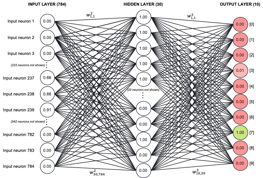
Weights: As we have 784 pixels in total for each image, we will also have 784 input neurons in our model. As 784 neurons would be too much to display here, I’ve skipped most of the neurons, and just shown some input neurons in the middle that are not just zeros (try to locate them in the GIF). In the hidden layer, I’ve chosen to have 30 hidden neurons (with 20 of them skipped in the image above to keep it simple). Then finally our output layer with 10 neurons corresponding to digits from 0 to 9. All of the neurons are connected with a weight from the very first input neuron to each of the neurons in the hidden layer. I.e. input neuron 1 is connected with a weight to each of the 30 neurons in the hidden layer — and the same is input neuron 2, etc., all the way to input neuron 784. Doing some simple math, this gives us a total of 30 x 784 = 23,520 weights from the input layer to the hidden layer. Each of these weights has a value assigned to them and together they decide each of the values in the hidden layer. The weights can be found in the excel file on the Parameters tab in area A1:AB870.
The same goes from the hidden layer to the output layer. This time we just have 30 neurons in the hidden layer however, which is each connected to just 10 output neurons, giving us just 30 x 10 = 300 weights this time. Much less, but still too many to show every single weight. If you don’t understand yet how it all interconnects, don’t worry, in the next section I’ll explain how it’s all put together — but first, we just need to understand biases. The weights can be found in the excel file on the Parameters tab in area A871:A1180.
Terminology: a weight from neuron 1 in layer 1 to neuron 1 in layer 2 can be written as seen on the picture just above the very first weight, which corresponds to the value of cell A2 on the parameters tab of the Excel file. The weight from the very last input neuron to the very last neuron in the hidden layer, i.e. w(2–1,784) in the lower bottom part of the weights to the left can be found in cell AB870. Weight w(3–1,1) in cell A872 and weight w(30–10,30) in cell A1180. It is not that important where each weight is located — just for you to have an idea how to navigate around in the Excel sheet.
Biases: Besides weights, a neural network also has biases, which is something that is added to the value for each of the hidden layers and the out layers. These biases are not shown in the illustration above, but can be found in the excel file on the Parameters tab in area A1181:A1222.
Note: you may be thinking, so where do these values for the weights and biases come from? Remember, this is a trained neural network, which means that we will not go through how to get these weights, but just how to use them. If you’re curious to know how to train a neural network, I recommend you to study Michael Nielsen’s resources who uses the same dataset — and who has inspired me a lot to study AI.
Understanding the calculations
Now that we have the weights and biases in place, let’s try to figure out how to calculate what we need. It is actually not that complicated, we just need to calculate 40 different numbers (30 for the hidden layers and 10 for the output layers). The output layer depends however on the calculations in the hidden layer (if we had more hidden layers each layer would always be dependent on the layer just before it). To keep the mathematical notation simple, let’s write the value of the hidden neuron like this:

Note: the superscript 2 does not means we are squaring the value, it simply means from the first layer (subscript 1) to the second layer (superscript 2).
For those of you who are familiar with the sigmoid function, this is basically it. However, in neural networks it’s often referred to as an activation function. Let’s just quickly clarify what the letters in the equation above mean.
- e (simply Euler’s number, a constant approximately equal to 2.71828)
- I (the input neurons, i.e the value of each of the 784 pixels — same values for each hidden neuron)
- W (the weights from each of the input pixels to the first neuron of the hidden layer — also 784 values, but new values for each hidden neuron, i.e. total of 23,520 different values)
- B (the bias term belonging to the first neuron of the hidden layer — for the first hidden neuron this corresponds to cell A1182 which has a value of 0.43)
Notice that we are taking the dot-product between the input neurons and the weights. Remember, we have 784 input neurons and 784 corresponding weights (with the weights changing for each neuron in the hidden layer). The value of input neuron 1 and weight from input neuron 1 to neuron in the hidden layer are multiplied — we do this for each of them and take the sum of the product, to which we add the bias term. The negative value of this is taken as the power of Euler’s number, to which we add 1. We then finally divide 1 by the sum of these numbers. If we had to provide an example with all the numbers, it would be very long — but check cell AD2 which has the final value for this number — which in Excel can be written as:
=1/(1+EXP(-(SUMPRODUCT(number;weight_1_1)+INDEX(bias_1;1)))) Where the ‘number’ is the array of the value of the pixels from the number, and ‘weight_1_1’ represents the weights from the input layer to the first neuron in the hidden layer. I’ve named the arrays so the formulas make more sense — if you want to explore the arrays, go to Formulas->Define Name in Excel to see what the arrays represent.
The value of the first hidden neuron is shown in the image as 1.00, but it this is just due to rounding. It’s really 0.99676789. So what does that really mean? There is not really any easy way to interpret this — the good thing is however that it works.
Going back to the equation, we basically just have to apply this for each of the neurons in the hidden layer (30 in total), and we thus have the values of our hidden layer. It’s actually not very different doing this for the final output layer, the only difference is just that we do no longer use the 784 pixels as our inputs anymore — we use the values for each of the neurons in the hidden layers, i.e. the values we just calculated. Each of these neurons in the hidden layers has its own weight (A871:A1180) assigned to them (just as in the picture), as well as each of the neurons in the output layer has its own bias (A1212:A1222) attached to them. You find the final calculations for the output layer in cells AE1:AE11.
Draw your own numbers
Try to go to the ‘Draw’ tab of the Excel file to draw your own numbers and see how the neural network classifies your own digits. Hopefully it should do so a bit better — but can still be challenging, try to draw a 7.

I hope this short article and the Excel file has been helpful for you to understand neural network better. Feel free to leave your comments or questions. Maybe I will make a new post in the future how to train a neural network and derive the weights and biases.