Getting Started
Develop an Image-to-Image Translation Model to Capture Local Interactions in Mechanical Networks (GAN)
Generative Adversarial Network used to automatically draw linkages on images of various mechanical networks.
Overview
Metamaterials are materials whose mechanical properties rely on their structure, which grants them modes of deformation that are not found in conventional systems. A popular model for metamaterials consist of building blocks connected to one another via mechanical linkages, which defines the structure of the material. These are called mechanical networks. Two mechanical networks differ from one another depending on:
- how the blocks are connected. This will define the class of system we deal with (e.g. Kagome system, square, triangular, etc..).
- how the blocks are distributed in space, i.e. how close there are from one another.
In other words, both position and connectivity of the blocks are critical to know in order to classify the system and grasp its mechanical properties. Often enough, mechanical networks are visually described by a lattice representation: points (also known as sites) represent the building blocks, and are connected by bonds (a.k.a edges). A typical mechanical network often considered in the research community is the Kagome system, drawn below.

Problem Statement and Methodology
In some instances, specially when dealing with microscopic metamaterials, a user/researcher will deal with images of the building blocks only (the points), the connecting bonds being too small to be detected and yet still present and contributing to the mechanical properties of the system. This project is intended to use deep learning and neural networks to automatically draw the bond connections on images that contain the points only.

To that end, we will use Dr. Jason Brownless’ article on how to develop a Generative Adversarial Network (GAN) that serves as an image-to-image algorithm. By only training on 90 of images of three different mechanical networks — Kagome, triangular and square lattices — the model successfully draws connecting bonds on images of unseen systems. While the results are pretty astonishing, the architecture of the model is equally fascinating to learn about.
The data used to train/test/validate the model consists of images generated by Mathematica, a program often used in the research and academic communities. Each image provided actually consists of a pair of images, respectively the same system (i.e. the points are identically spatially distributed) with and without the bonds. We then select 30 randomly generated Kagome lattices, along with 30 more square and 30 more triangular lattices:


The code used here is obviously written Python and relies principally on the package Keras (along with the usual suspects numpy and matplotlib) to build and train the multiple neural networks. The notebook (which can be found here) is written via Google Colab which allows us to take advantage of Google’s GPU services.
Generative Adversarial Network (GAN)
The GAN’s architecture consists of two main models that train together in an adversarial manner — the discriminator and the generator — along with other features that bind and train them together
The discriminator
The discriminator is a deep Convolutional Neural Network (CNN) that takes an image shape and performs conditional-image classification. In summary, it takes the source image (without bonds) and the target image (with bonds) and classifies if the target is the real translation of the source. Prior to be fed to the network, the two images are concatenated into a single one.

The deep CNN consists of 6 layers, each one of them downsizing the output image of the previous layer, to output a score which serves as the classification metric.
The generator
The generator follows a U-net architecture and consists of three sections: the encoder (contraction), the bottleneck and the decoder (expansion).

- The encoder section consists of multiple blocks that downsample the input image. Each block is a convolution layer with an ever-so-increasing number of filters.
- On the contrary, the decoder consists of several expansion blocks, with a number of filters ever-so-decreasing. Importantly enough, the input of each expanding layer features both the output of the previous expanding block AND the output of corresponding contracting block. This ensures the features learned during the encoding phase are re-used to reconstruct the image in the decoding one.
- The bottleneck section connects the encoding and decoding sections.
The composite and train models
The Generative Adversarial Network (GAN) is a composite model which consists of both discriminator and generator at once. While the generator updates its weights via the discriminator, the discriminator isn’t trained and updates its weights “on its own”. The key feature is that the weights update for the discriminator needs to be slow compared to the generator, so the generator learns rapidly to draw the bonds.
Each training step consists of using the composite model along with “real” images from the training data and “fake” generated images from the generator. The idea is that a combination of real target and fake generated images, respectively classified as 1 and 0, will help the generator build a model that converges faster toward a solution.

There are many tunable parameters and complex designs at stake in this model. To keep this article simple and readable, I purposefully omit to mention the complexity of the code, but invite the reader to checkout my Github repository for more details.
Results
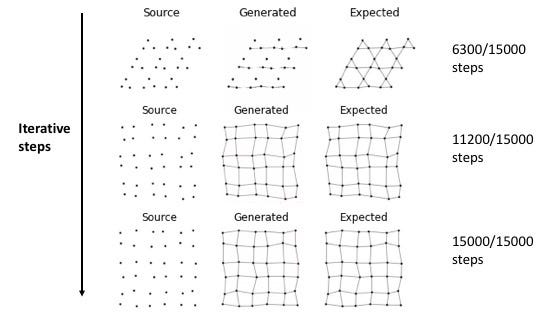
We train the model on 90 images, split in 3 batches, meaning there are 30 images drawn at random in each batch per epoch. We choose to train the model on 500 epochs, meaning there is a total of 500 x 30 = 15,000 iterative steps. While training the model on a local machine would likely take up to a day, Google GPU’s quicken the process to less than 2 hours! Through the iterative process, we display what generated images of samples drawn at random from the training dataset look like:

Testing the model against its own training set is a poor choice to check for its performance, but it gives us an idea on how well the generating feature is carried out. Therefore, we need to also display how the model performs on unseen data:

Originally, my goal was to build the model against the Kagome class only. I then decided to expand the range of applications of the model to include square and triangular lattices:
- top row: the 1st model is trained only on images of Kagome systems and clearly struggles in drawing the connections for square and triangular
- bottom row: the 2nd model incorporates all three lattices and produces better and more significant results
Very importantly, in addition to drawing the bonds, the 2nd model also maintains the position of the points on the generated figures, a critical property which must remain invariant, since the position of these points dictate the mechanical properties of the system (as mentioned above).
Conclusion and Further Improvements
By training on 90 pairs of images only, the model can take unseen images of partially complete mechanical networks and plot the proper bond connectivity, a critical feature to understand the mechanics of the system. In doing so, the model does not change the fundamental properties of the material(the position of the points/blocks) and provides additional information for the researcher. Excitingly enough, the model is able to distinguish and carry out its image-to-image translation feature on not just one, but three mechanical systems: Kagome, square and triangular lattices.
While this is a satisfying result, many things can be done to improve the model’s performance. In particular, we can:
- train the model on a larger set of images and for a longer time (more epochs)
- expand the training batch to include additional classes of metamaterials, specially the more complex structures, like those where the average number of connections per site is greater than what we’ve seen so far
References and Acknowledgments
Again, code, slides and reports can be found here. All images (unless indicated otherwise) were made by the author. I’d like to particularly thank my mentor at Springboard, Lucas Allen, for his guidance through this project. I also would like to thank Dr. Brownlee for his multiple online tutorials in helping developers build Machine Learning models.
[1] J. Brownlee, How to Develop a Pix2Pix GAN for Image-to-Image Translation (2020), Machine Learning Mystery


