Climate Data Science
A Quick Introduction to Google Earth Engine
A small glimpse of the wealth of satellite and climate data in the Cloud.
Google Earth Engine (GEE) is a platform for cloud-based geospatial applications with tons of data from satellites, including the ones from the famous Landsat program to several climate datasets. The best thing is that the platform is available to anyone with enough interest and a relatively decent internet connection, making environmental processing easy to use and available to those who need it the most.
There are several ways to use GEE and each one has its advantages and disadvantages. While the Javascript-based Code Editor is probably the most used tool and the Explorer is perfect for a casual look, here you’ll put your hands on the Python API. In the meanwhile, feel free to explore the available datasets and many successful case studies.
Signing Up
Basically, any person with a Google account can sign up to use GEE and the installation of the necessary packages is quite straightforward. After signing up, you can install the Earth Engine Python API with pip:
pip install earthengine-apiAfter that, you need to set up your authentication credentials on your computer. The entire (not so long) process is described in detail in the manual and you’re encouraged to test the installation as described in the end. After these quick steps, you’re ready to go with an immense collection of datasets ready to be explored.
Importing the packages
The Earth Engine Package is simply called ee, and with that, you can start to set up your toolbox. Apart from ee, here in this tutorial, you’ll also need Folium for interactive maps and geehydro, which is intended to be a package for inundation dynamics in the GEE platform but is extraordinarily useful as it emulates some of the functions from the Javascript API. You can install these other packages with pip as well:
pip install folium
pip install geehydro
To import all the packages:
import ee
import folium
import geehydrofrom datetime import datetime as dt
from IPython.display import Image
When you use the API, the first thing you need to do is to initialize the connection to the server:
# initialize the connection to the server
>>> ee.Initialize()
Select a region in the world
With satellite imagery you can investigate any spot on Earth, even remote places where you could never set foot on (or at least you shouldn’t). In this tutorial, you’ll explore the recent conditions in the Ituna/Itatá Indigenous Land in the Brazilian state of Pará. This protected land is home to a few isolated indigenous tribes and is one of the places in the Amazon where mining, logging and ranching are absolutely illegal practices. Unfortunately, according to the Brazilian National Institute of Space Research (INPE) this place also became the most affected of all during last year by the advance of the agricultural border in Brazil, menacing the lives of the tribes who live there and the biodiversity within.
Aided by Folium, you can take a look at where this distant place is:
# the Ituna/Itatá Indigenous Land in Brazil.
Ituna_map = folium.Map(location=[-4.06738, -52.034], zoom_start=10)
>>> Ituna_map
The Landsat 8 Collection
Landsat 8 is the most recent addition to the long-running Landsat Program and it’s been in orbit since 2013, continuously estimating the land-surface conditions around the globe. Applications of Landsat imagery are widely known and well-established in the fields of agronomy, environmental conservation and changes related to land-use.
There are several technical details about Landsat 8, but the basics you should know is that it collects multispectral spatial information in a medium resolution, with bands a range of 15 to 100 meters resolutions in 11 different bands of the electromagnetic spectrum. It also has a revisit time of 16 days, which means you have a new image of a particular place every 16 days cycle.
With ee, you can have access to the entire Landsat 8 collection with a single line of code:
landsat = ee.ImageCollection("LANDSAT/LC08/C01/T1_SR")Each collection has its own id and you can find them in the GEE catalog. Above, the EE snippet id for the Landsat 8 Surface Reflectance Tier 1 product is "LANDSAT/LC08/C01/T1_SR" as described in the catalog.
This will get you the entire collection of imagery of the entire world, so you’ll have to tailor it out according to both your area and time of interests. For the area, you’ll set up a rectangle around the Ituna/Itatá Land using latitude/longitude information with ee.Geometry.Rectangle:
# setting the Area of Interest (AOI)
Ituna_AOI = ee.Geometry.Rectangle([-51.84448, -3.92180,
                                   -52.23999, -4.38201])
The .filterBounds() method allows you to select the AOI you defined above:
# filter area
landsat_AOI = landsat.filterBounds(Ituna_AOI)
Another detail is that you might not be interested in the entire time span of the collection, but in a particular period. For the Ituna/Itatá Land, you’ll select a brief period of time during the dry season in the region in 2019. Why the dry season? Clouds are a major problem for satellite imagery analysis and in the Amazon, this problem is severely increased, so selecting months without intense rainfall and cloud cover is a nice strategy. Also, these are the months where deforestation goes rampant and the (human-induced) fire season starts.
# choose dates
landsat = landsat.filterDate('2019-07-01','2019-12-01')
A bit of meta-data
You can easily .getInfo() about the Landsat collection above or any particular information you might be interested in. For the landsat_AOI collection tailored above, it will get you all the information there’s to know about it, which could be a little messy and too technical.
>>> landsat_AOI.getInfo()
It’s possible to be more selective and filter out the information you don’t want. Assuming you just need to know how many images from Landsat you got from the period of time selected above, simply do:
>>> print('Total number:', landsat_AOI.size().getInfo())
Total number: 9
Another example is to show how each band from Landsat 8 is named — something useful for the next steps:
# the names of each Landsat 8 band
>>> landsat_AOI.first().bandNames().getInfo()['B1',
 'B2',
 'B3',
 'B4',
 'B5',
 'B6',
 'B7',
 'B10',
 'B11',
 'sr_aerosol',
 'pixel_qa',
 'radsat_qa']
Choosing an Image
It’s possible to be more selective and set up the collection according to a particular criterion. In this tutorial, you’ll select the least cloudy image from the landsat_AOI collection according to its 'CLOUD_COVER' id.
# the least cloudy image
least_cloudy = ee.Image(landsat_AOI.sort('CLOUD_COVER').first())# how cloudy is it?
>>> print('Cloud Cover (%):', least_cloudy.get('CLOUD_COVER').getInfo())
Cloud Cover (%): 0
Conveniently so, satellite imagery with 0% of 'CLOUD_COVER' in the Amazon is something hard to see. This one is perfect, but when it was taken?
# when was this image taken?
date = ee.Date(least_cloudy.get('system:time_start'))
time = date.getInfo()['value']/1000.>>> dt.utcfromtimestamp(time).strftime('%Y-%m-%d %H:%M:%S')'2019-08-11 13:36:22'
August is one of the driest months of the dry season in the Amazon, so it comes as no surprise that it has 0% 'CLOUD_COVER'.
Visualizing the Satellite Imagery
A common practice when doing an analysis with satellite imagery is to combine different bands. Since each band represents a portion of the electromagnetic spectrum, combining them allows different views of the same surface due to the spectral signature of types of vegetation, water, soil and things like that. The easiest one is the Red-Green-Blue (RGB) composite and when using Landsat 8 imagery, you’ll need to use Bands 4 (Red), 3 (Green) and 2 (Blue).
The Javascript-based code editor easily allows interactive visualization using Map.AddLayer(), but unfortunately, this is not available for the standard Python API. A simple, static map can be made with both the .getThumbURL() module from ee and the native .display() module from IPython:
parameters = {'min': 0,
              'max': 1000,
              'dimensions': 512,
              'bands': ['B4', 'B3', 'B2'],
              'region': Ituna_AOI}

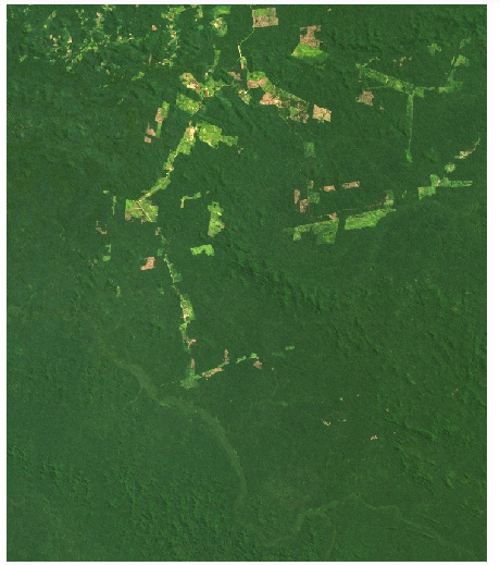
>>> Image(url = least_cloudy.getThumbUrl(parameters))
The parameters variable stores the options you can explore when analyzing satellite imagery with ee. It works in the same way as the Javascript API and you’re encouraged to combine different bands and tweak it out to get different visualizations of the same data.
For the purpose of the tutorial, the simple RGB composite does justice to investigate the advance of illegal logging and other practices in a land where this is not supposed to happen. In the image above, everything that is not in a strong green tone is against the law. This happened in mid-August of 2019, but as February of our current year of 2020 the situation is, unfortunately, much worse.
Normalized Difference Vegetation Index (NDVI)
There are more quantitative ways to investigate the land-use changes and deforestation. Perhaps the best-known method is the use of the Normalized Difference Vegetation Index (NDVI), widely present in several land management, agriculture and conservation studies.
NDVI needs information from the Near-Infrared (NIR) and Visible (VIS) bands, which for Landsat 8 are the bands 5 and 4. The calculation is simply NDVI = (NIR-VIS)/(NIR+VIS), but the insights from it can be huge. It ranges from -1 to 1 or 0 to 1 in some more classic studies. A pixel with a negative or 0 value could be many things, like a river body or a severely degraded land, while a pixel close to 1 is certainly a dense portion of vegetation.
Since this is a common practice, you can quickly calculate any Normalized Difference Index (NDVI is not the only one)with .normalizedDifference:
ndvi = least_cloudy.normalizedDifference(['B5', 'B4'])After this, you’ll certainly wish to visualize it on a pretty map. While you already know the native way, geehydro allows you to plot an interactive map with Folium just like the Code Editor does with Map.AddLayer():
palette = ['red', 'yellow', 'green']ndvi_parameters = {'min': 0,
                   'max': 1,
                   'dimensions': 512,
                   'palette': palette,
                   'region': Ituna_AOI}Ituna_map.addLayer(ndvi, ndvi_parameters)
Ituna_map

The use of geehydro allows an even greater degree of reproducibility between the Javascript and Python API, building a large bridge between often two separate kinds of people. If you don’t know a word about Javascript, now you can understand the code in the several GEE tutorials available around the internet.
Final words
GEE is an excellent tool to learn how to use satellite imagery for good and the possibilities are huge. Land-use changes studies, sustainable farming and monitoring of sensitive areas like the Ituna/Itatá are available for anyone with a good internet connection and enough interest to go for it. The flexible Python API and the usefulness of geehydro can be combined to quickly set up the platform to use. With it, tons of different datasets and a wealth of information ready to be discovered. What a time to be alive.
The interactive Jupyter Notebook for this tutorial is freely available in my Climate Data Science repository.


