A Comprehensive Overview of Gaussian Splatting

Everything you need to know about the new trend in the field of 3D representations

Gaussian splatting is a method for representing 3D scenes and rendering novel views introduced in “3D Gaussian Splatting for Real-Time Radiance Field Rendering”¹. It can be thought of as an alternative to NeRF²-like models, and just like NeRF back in the day, Gaussian splatting led to lots of new research works that chose to use it as an underlying representation of a 3D world for various use cases. So what’s so special about it and why is it better than NeRF? Or is it, even? Let’s find out!

Table of contents:

• TL;DR
• Representing a 3D world
• Image formation model & rendering
• Optimization
• View-dependant colors with SH
• Limitations
• Where to play with it

TL;DR

First and foremost, the main claim to fame of this work was the high rendering speed as can be understood from the title. This is due to the representation itself which will be covered below and thanks to the tailored implementation of a rendering algorithm with custom CUDA kernels.

Figure 1: A side-by-side comparison of previous high-quality representations and Gaussian Splatting (marked as “Ours”) in terms of rendering speed (fps), training time (min), and visual quality (Peak signal-to-noise ratio, the higher the better) [Source: taken from [1]]

Additionally, Gaussian splatting doesn’t involve any neutral network at all. There isn’t even a small MLP, nothing “neural”, a scene is essentially just a set of points in space. This in itself is already an attention grabber. It is quite refreshing to see such a method gaining popularity in our AI-obsessed world with research companies chasing models comprised of more and more billions of parameters. Its idea stems from “Surface splatting”³ (2001) so it sets a cool example that classic computer vision approaches can still inspire relevant solutions. Its simple and explicit representation makes Gaussian splatting particularly interpretable, a very good reason to choose it over NeRFs for some applications.

Representing a 3D world

As mentioned earlier, in Gaussian splatting a 3D world is represented with a set of 3D points, in fact, millions of them, in a ballpark of 0.5–5 million. Each point is a 3D Gaussian with its own unique parameters that are fitted per scene such that renders of this scene match closely to the known dataset images. The optimization and rendering processes will be discussed later so let’s focus for a moment on the necessary parameters.

Figure 2: Centers of Gaussian (means) [Source: taken from Dynamic 3D Gaussians⁴]

Each 3D Gaussian is parametrized by:

• Mean μ interpretable as location x, y, z;
• Covariance Σ;
• Opacity σ(𝛼), a sigmoid function is applied to map the parameter to the [0, 1] interval;
• Color parameters, either 3 values for (R, G, B) or spherical harmonics (SH) coefficients.

Two groups of parameters here need further discussion, a covariance matrix and SH. There is a separate section dedicated to the latter. As for the covariance, it is chosen to be anisotropic by design, that is, not isotropic. Practically, it means that a 3D point can be an ellipsoid rotated and stretched along any direction in space. It could have required 9 parameters, however, they cannot be optimized directly because a covariance matrix has a physical meaning only if it’s a positive semi-definite matrix. Using gradient descent for optimization makes it hard to pose such constraints on a matrix directly, that is why it is factorized instead as follows:

Such factorization is known as eigendecomposition of a covariance matrix and can be understood as a configuration of an ellipsoid where:

• S is a diagonal scaling matrix with 3 parameters for scale;
• R is a 3x3 rotation matrix analytically expressed with 4 quaternions.

The beauty of using Gaussians lies in the two-fold impact of each point. On one hand, each point effectively represents a limited area in space close to its mean, according to its covariance. On the other hand, it has a theoretically infinite extent meaning that each Gaussian is defined on the whole 3D space and can be evaluated for any point. This is great because during optimization it allows gradients to flow from long distances.⁴

The impact of a 3D Gaussian i on an arbitrary 3D point p in 3D is defined as follows:

Figure 3: An influence of a 3D Gaussian i on a point p in 3D [Source: Image by the author]

This equation looks almost like a probability density function of the multivariate normal distribution except the normalization term with a determinant of covariance is ignored and it is weighting by the opacity instead.

Image formation model & rendering

Image formation model

Given a set of 3D points, possibly, the most interesting part is to see how can it be used for rendering. You might be previously familiar with a point-wise 𝛼-blending used in NeRF. Turns out that NeRFs and Gaussian splatting share the same image formation model. To see this, let’s take a little detour and re-visit the volumetric rendering formula given in NeRF² and many of its follow-up works (1). We will also rewrite it using simple transitions (2):

You can refer to the NeRF paper for the definitions of σ and δ but conceptually this can be read as follows: color in an image pixel p is approximated by integrating over samples along the ray going through this pixel. The final color is a weighted sum of colors of 3D points sampled along this ray, down-weighted by transmittance. With this in mind, let’s finally look at the image formation model of Gaussian splatting:

Indeed, formulas (2) and (3) are almost identical. The only difference is how 𝛼 is computed between the two. However, this small discrepancy turns out extremely significant in practice and results in drastically different rendering speeds. In fact, it is the foundation of the real-time performance of Gaussian splatting.

To understand why this is the case, we need to understand what f^{2D} means and which computational demands it poses. This function is simply a projection of f(p) we saw in the previous section into 2D, i.e. onto an image plane of the camera that is being rendered. Both a 3D point and its projection are multivariate Gaussians so the impact of a projected 2D Gaussian on a pixel can be computed using the same formula as the impact of a 3D Gaussian on other points in 3D (see Figure 3). The only difference is that the mean μ and covariance Σ must be projected into 2D which is done using derivations from EWA splatting⁵.

Means in 2D can be trivially obtained by projecting a vector μ in homogeneous coordinates (with extra 1 coordinate) into an image plane using an intrinsic camera matrix K and an extrinsic camera matrix W=[R|t]:

This can be also written in one line as follows:

Here “z” subscript stands for z-normalization. Covariance in 2D is defined using a Jacobian of (4), J:

The whole process remains differentiatable, and that is of course crucial for optimization.

Rendering

The formula (3) tells us how to get a color in a single pixel. To render an entire image, it’s still necessary to traverse through all the HxW rays, just like in NeRF, however, the process is much more lightweight because:

• For a given camera, f(p) of each 3D point can be projected into 2D in advance, before iterating over pixels. This way, when a Gaussian is blended for a few nearby pixels, we won’t need to re-project it over and over again.
• There is no MLP to be inferenced H·W·P times for a single image, 2D Gaussians are blended onto an image directly.
• There is no ambiguity in which 3D point to evaluate along the ray, no need to choose a ray sampling strategy. A set of 3D points overlapping the ray of each pixel (see N in (3)) is discrete and fixed after optimization.
• A pre-processing sorting stage is done once per frame, on a GPU, using a custom implementation of differentiable CUDA kernels.

The conceptual difference can be seen in Figure 4:

Figure 4: A conceptual difference between NeRF and GS, Left: Query a continuous MLP along the ray, Right: Blend a discrete set of Gaussians relevant to the given ray [Source: Image by the author]

The sorting algorithm mentioned above is one of the contributions of the paper. Its purpose is to prepare for color rendering with the formula (3): sorting of the 3D points by depth (proximity to an image plane) and grouping them by tiles. The first is needed to compute transmittance, and the latter allows to limit the weighted sum for each pixel to α-blending of the relevant 3D points only (or their 2D projections, to be more specific). The grouping is achieved using simple 16x16 pixel tiles and is implemented such that a Gaussian can land in a few tiles if it overlaps more than a single view frustum. Thanks to sorting, the rendering of each pixel can be reduced to α-blending of pre-ordered points from the tile the pixel belongs to.

Figure 5: View frustums, each corresponding to a 16x16 image tile. Colors have no special meaning. The result of the sorting algorithm is a subset of 3D points within each tile sorted by depth. [Source: Based on the plots from here]

Optimization

A naive question might come to mind: how is it even possible to get a decent-looking image from a bunch of blobs in space? And well, it is true that if Gaussians aren’t optimized properly, you will get all kinds of pointy artifacts in renders. In Figure 6 you can observe an example of such artifacts, they look quite literally like ellipsoids. The key to getting good renders is 3 components: good initialization, differentiable optimization, and adaptive densification.

Figure 6: An example of renders of an under-optimized scene [Source: Image by the author]

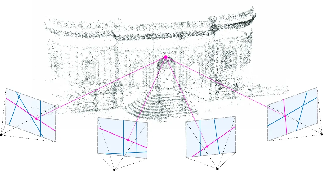
The initialization refers to the parameters of 3D points set at the start of training. For point locations (means), the authors propose to use a point cloud produced by SfM (Structure from Motion), see Figure 7. The logic is that for any 3D reconstruction, be it with GS, NeRF, or something more classic, you must know camera matrices so you would probably run SfM anyway to obtain those. Since SfM produces a sparse point cloud as a by-product, why not use it for initialization? So that’s what the paper suggests. When a point cloud is not available for whatever reason, a random initialization can be used instead, under the risk of a potential loss of the final reconstruction quality.

Figure 7: A sparse 3D point cloud produced by SfM, means initialization [Source: Taken from here]

Covariances are initialized to be isotropic, in other words, 3D points begin as spheres. The radiuses are set based on mean distances to neighboring points such that the 3D world is nicely covered and has no “holes”.

After init, a simple Stochastic Gradient Descent is used to fit everything properly. The scene is optimized for a loss function that is a combination of L1 and D-SSIM (structural dissimilarity index measure) between a ground truth view and a current render.

However, that’s not it, another crucial part remains and that is adaptive densification. It is launched once in a while during training, say, every 100 SGD steps and its purpose is to address under- and over-reconstruction. It’s important to emphasize that SGD on its own can only do as much as adjust the existing points. But it would struggle to find good parameters in areas that lack points altogether or have too many of them. That’s where adaptive densification comes in, splitting points with large gradients (Figure 8) and removing points that have converged to very low values of α (if a point is that transparent, why keep it?).

Figure 8: Adaptive densification. A toy example of fitting a bean shape that we’d like to render with a few points. [Source: Taken from [1]]

View-dependant colors with SH

Spherical harmonics, SH for short, play a significant role in computer graphics and were first proposed as a way to learn a view-dependant color of discrete 3D voxels in Plenoxels⁶. View dependence is a nice-to-have property that improves the quality of renders since it allows the model to represent non-Lambertian effects, e.g. specularities of metallic surfaces. However, it is certainly not a must since it’s possible to make a simplification, choose to represent color with 3 RGB values, and still use Gaussian splatting like it was done in [4]. That is why we are reviewing this representation detail separately after the whole method is laid out.

SH are special functions defined on the surface of a sphere. In other words, you can evaluate such a function for any point on the sphere and get a value. All of these functions are derived from this single formula by choosing positive integers for ℓ and −ℓ ≤ m ≤ ℓ, one (ℓ, m) pair per SH:

While a bit intimidating at first, for small values of l this formula simplifies significantly. In fact, for ℓ = 1, Y = ~0.282, just a constant on the whole sphere. On the contrary, higher values of ℓ produce more complex surfaces. The theory tells us that spherical harmonics form an orthonormal basis so each function defined on a sphere can be expressed through SH.

That’s why the idea to express view-dependant color goes like this: let’s limit ourselves to a certain degree of freedom ℓ_max and say that each color (red, green, and blue) is a linear combination of the first ℓ_max SH functions. For every 3D Gaussian, we want to learn the correct coefficients so that when we look at this 3D point from a certain direction it will convey a color the closest to the ground truth one. The whole process of obtaining a view-dependant color can be seen in Figure 9.

Figure 9: A process of obtaining a view-dependant color (red component) of a point with ℓ_max = 2 and 9 learned coefficients. A sigmoid function maps the value into the [0, 1] interval. Oftentimes, clipping is used instead [Source: Image by the author]

Limitations

Despite the overall great results and the impressive rendering speed, the simplicity of the representation comes with a price. The most significant consideration is various regularization heuristics that are introduced during optimization to guard the model against “broken” Gaussians: points that are too big, too long, redundant, etc. This part is crucial and the mentioned issues can be further amplified in tasks beyond novel view rendering.

The choice to step aside from a continuous representation in favor of a discrete one means that the inductive bias of MLPs is lost. In NeRFs, an MLP performs an implicit interpolation and smoothes out possible inconsistencies between given views, while 3D Gaussians are more sensitive, leading back to the problem described above.

Furthermore, Gaussian splatting is not free from some well-known artifacts present in NeRFs which they both inherit from the shared image formation model: lower quality in less seen or unseen regions, floaters close to an image plane, etc.

The file size of a checkpoint is another property to take into account, even though novel view rendering is far from being deployed to edge devices. Considering the ballpark number of 3D points and the MLP architectures of popular NeRFs, both take the same order of magnitude of disk space, with GS being just a few times heavier on average.

Where to play with it

No blog post can do justice to a method as well as just running it and seeing the results for yourself. Here is where you can play around:

• gaussian-splatting — the official implementation with custom CUDA kernels;
• nerfstudio —yes, Gaussian splatting in nerfstudio. This is a framework originally dedicated to NeRF-like models but since December, ‘23, it also supports GS;
• threestudio-3dgs — an extension for threestudio, another cross-model framework. You should use this one if you are interested in generating 3D models from a prompt rather than learning an existing set of images;
• UnityGaussianSplatting — if Unity is your thing, you can port a trained model into this plugin for visualization;
• gsplat — a library for CUDA-accelerated rasterization of Gaussians that branched out of nerfstudio. It can be used for independent torch-based projects as a differentiatable module for splatting.

Have fun!

Acknowledgments

This blog post is based on a group meeting in the lab of Dr. Tali Dekel. Special thanks go to Michal Geyer for the discussions of the paper and to the authors of [4] for a coherent summary of Gaussian splatting.

References

1. Kerbl, B., Kopanas, G., Leimkühler, T., & Drettakis, G. (2023). 3D Gaussian Splatting for Real-Time Radiance Field Rendering. SIGGRAPH 2023.
2. Mildenhall, B., Srinivasan, P. P., Tancik, M., Barron, J. T., Ramamoorthi, R., & Ng, R. (2020). NeRF: Representing Scenes as Neural Radiance Fields for View Synthesis. ECCV 2020.
3. Zwicker, M., Pfister, H., van Baar, J., & Gross, M. (2001). Surface Splatting. SIGGRAPH 2001
4. Luiten, J., Kopanas, G., Leibe, B., & Ramanan, D. (2023). Dynamic 3D Gaussians: Tracking by Persistent Dynamic View Synthesis. International Conference on 3D Vision.
5. Zwicker, M., Pfister, H., van Baar, J., & Gross, M. (2001). EWA Volume Splatting. IEEE Visualization 2001.
6. Yu, A., Fridovich-Keil, S., Tancik, M., Chen, Q., Recht, B., & Kanazawa, A. (2023). Plenoxels: Radiance Fields without Neural Networks. CVPR 2022.