You have probably heard of the Swiss army knife. If not, just take a look at the image below. It contains many blades and tools. Each one is specialized at a particular task. In some cases, different blades can do the same task but with a different degree of performance.

I think of the Machine Learning algorithms as Swiss army knife. There are many different algorithms. Certain tasks require to use a particular algorithm whereas some tasks can be done with many different algorithms. The performance might change depending on the characteristics of the task and data.
In this post, I will share 16 tips that I think will help you better understand the algorithms. My goal is not to explain how algorithms work in detail. I will rather give some tips or details about them.
Some tips will be more general and not be focused on a particular algorithm. For instance, log loss is a cost function that is related to all classification algorithm.
I will assume you have a basic understanding of the algorithm. Even if you don’t, you can pick some details that will help you later on.
Let’s start.
1. C parameter of support vector machine (SVM)
C parameter of SVM adds a penalty for each misclassified data point. If c is small, penalty for a misclassified point is low so a decision boundary with a large margin is chosen at the expense of a greater number of misclassifications.
If c is large, SVM tries to minimize the number of misclassified examples due to high penalty which results in a decision boundary with a smaller margin. Penalty is not same for all misclassified examples. It is directly proportional to the distance to decision boundary.
2. Gamma parameter of SVM with RBF kernel
Gamma parameter of SVM with RBF kernel controls the distance of influence of a single training point. Low values of gamma indicates a large similarity radius which results in more points being grouped together.
For high values of gamma, the points need to be very close to each other in order to be considered in the same group (or class). Therefore, models with very large gamma values tend to overfit.
3. What makes logistic regression a linear model
The basis of logistic regression is the logistic function, also called the sigmoid function, which takes in any real valued number and maps it to a value between 0 and 1.

It is a non-linear function but logistic regression is a linear model.
Here is how we get to a linear equation from the sigmoid function:

Taking the natural log of both sides:

In equation (1), instead of x, we can use a linear equation z:

Then equation (1) becomes:

Assume y is the probability of positive class. If it is 0.5, then the right hand side of the above equation becomes 0.
We have a linear equation to solve now.
4. The principal components in PCA
PCA (Principal component analysis) is a linear dimensionality reduction algorithm. The goal of PCA is to keep as much information as possible while reducing the dimensionality (number of features) of a dataset.
The amount of information is measured by the variance. Features with high variance tell us more about the data.
The principal components are linear combinations of the features of original dataset.
5. Random forests
Random forests are built using a method called bagging in which each decision trees are used as parallel estimators.
The success of a random forest highly depends on using uncorrelated decision trees. If we use same or very similar trees, overall result will not be much different than the result of a single decision tree. Random forests achieve to have uncorrelated decision trees by bootstrapping and feature randomness.

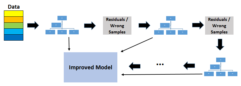
6. Gradient boosted decision trees (GBDT)
GBDT use boosting method to combine individual decision trees. Boosting means combining a learning algorithm in series to achieve a strong learner from many sequentially connected weak learners.
Each tree fits on the residuals from the previous tree. Unlike bagging, boosting does not involve bootstrap sampling. Every time a new tree is added, it fits on a modified version of initial data set.
7. Increasing the number of trees in Random Forest and GBDT
Increasing the number of trees in random forests does not cause overfitting. After some point, the accuracy of the model does not increase by adding more trees but it is also not negatively effected by adding excessive trees. You still do not want to add unnecessary amount of trees due to computational reasons but there is no risk of overfitting associated with the number of trees in random forests.
However, the number of trees in gradient boosting decision trees is very critical in terms of overfitting. Adding too many trees will cause overfitting so it is important to stop adding trees at some point.
8. Hierarchical clustering vs K-means clustering
Hierarchical clustering does not require to specify the number of clusters beforehand. The number of clusters must be specified for k-means algorithm.
It always generates the same clusters whereas k-means clustering may result in different clusters depending on the how the centroids (center of cluster) are initiated.
Hierarchical clustering is a slower algorithm compared to k-means. It takes long time to run especially for large data sets.
9. Two key parameters of DBSCAN algorithm
DBSCAN is a clustering algorithm that works well with arbitrary shaped clusters. It is also an efficient algoritm to detect outliers.
Two key parameters of DBSCAN:
- eps: The distance that specifies the neighborhoods. Two points are considered to be neighbors if the distance between them are less than or equal to eps.
- minPts: Minimum number of data points to define a cluster.
10. Three different types of points in DBSCAN algorithm
Based on eps and minPts parameters, points are classified as core point, border point, or outlier:
- Core point: A point is a core point if there are at least minPts number of points (including the point itself) in its surrounding area with radius eps.
- Border point: A point is a border point if it is reachable from a core point and there are less than minPts number of points within its surrounding area.
- Outlier: A point is an outlier if it is not a core point and not reachable from any core points.

In this case, minPts is 4. Red points are core points because there are at least 4 points within their surrounding area with radius eps. This area is shown with the circles in the figure. The yellow points are border points because they are reachable from a core point and have less than 4 points within their neighborhood. Reachable means being in the surrounding area of a core point. The points B and C have two points (including the point itself) within their neighborhood (i.e. the surrounding area with a radius of eps). Finally N is an outlier because it is not a core point and cannot be reached from a core point.
11. Why is Naive Bayes called naive?
Naive bayes algorithm assumes that features are independent of each other and there is no correlation between features. However, this is not the case in real life. This naive assumption of features being uncorrelated is the reason why this algorithm is called "naive".
The assumption that all features are independent makes naive bayes algorithm very fast compared to complicated algorithms. **** In some cases, speed is preferred over higher accuracy.
It works well with high-dimensional data such as text classification, email spam detection.
12. What is log loss?
Log loss (i.e. cross-entropy loss) is a widely-used cost function for machine learning and deep learning models.
Cross-entropy quantifies the comparison of two probability distributions. In supervised learning tasks, we have a target variable that we are trying to predict. The actual distribution of the target variable and our predictions are compared using the cross-entropy. The result is the cross-entropy loss, also known as log loss.
13. How is log loss calculated?
For each prediction, the negative natural log of the predicted probability of true class is calculated. The sum of all these values give us the log loss.
Here is an example that will explain the calculation better.
We have a classification problem with 4 classes. The prediction of our model for a particular observations is as below:

The log loss that come from this particular observation (i.e. data point or row) is -log(0.8) = 0.223.
14. Why do we use log loss instead of classification accuracy?
When calculating the log loss, we take the negative of the natural log of predicted probabilities. The more certain we are at the prediction, the lower the log loss (assuming the prediction is correct).
For instance, -log(0.9) is equal to 0.10536 and -log(0.8) is equal to 0.22314. Thus, being 90% sure results in a lower log loss than being 80% sure.
The traditional metrics like classification accuracy, precision, and recall evaluates the performance by comparing the predicted class and actual class.
The following table shows the predictions of two different models on a relatively small set that consists of 5 observations.

Both models correctly classified 4 observations out of 5. Thus, in terms of classification accuracy, these models have the same performance. However, the probabilities reveal that Model 1 is more certain in the predictions. Thus, it is likely to perform better in general.
Log loss (i.e. cross-entropy loss) provide a more robust and accurate evaluation of classification models.
15. ROC curve and AUC
ROC curve summarizes the performance by combining confusion matrices at all threshold values. AUC turns the ROC curve into a numeric representation of performance for a binary classifier. AUC is the area under the ROC curve and takes a value between 0 and 1. AUC indicates how successful a model is at separating positive and negative classes.
16. Precision and recall
Precision and recall metrics take the classification accuracy one step further and allow us to get a more specific understanding of model evaluation. Which one to prefer depends on the task and what we aim to achieve.
Precision measures how good our model is when the prediction is positive. The focus of precision is positive predictions. It indicates how many of the positive predictions are true.
Recall measures how good our model is at correctly predicting positive classes. The focus of recall is actual positive classes. It indicates how many of the positive classes the model is able to predict correctly.
Conclusion
We have covered some basic information as well as some details about machine learning algorithms.
Some points are related to multiple algorithms such as the ones about log loss. These are also important because evaluating the models is just as important as implementing them.
All the machine learning algorithms are useful and efficient in certain tasks. Depending on the tasks you are working one, you can master a few of them.
However, it is valuable to have an idea about how each of these algorithms work.
Thank you for reading. Please let me know if you have any feedback.


