Difference between AlexNet, VGGNet, ResNet, and Inception

In this tutorial, I will quickly go through the details of four of the famous CNN architectures and how they differ from each other by explaining their W3H (When, Why, What, and How)

AlexNet

When?

• The Alan Turing Year
• The year of Sustainable Energy for All
• London Olympics

Why? AlexNet was born out of the need to improve the results of the ImageNet challenge. This was one of the first Deep convolutional networks to achieve considerable accuracy on the 2012 ImageNet LSVRC-2012 challenge with an accuracy of 84.7% as compared to the second-best with an accuracy of 73.8%. The idea of spatial correlation in an image frame was explored using convolutional layers and receptive fields.

What? The network consists of 5 Convolutional (CONV) layers and 3 Fully Connected (FC) layers. The activation used is the Rectified Linear Unit (ReLU). The structural details of each layer in the network can be found in the table below.

Alexnet Block Diagram (source:oreilly.com)

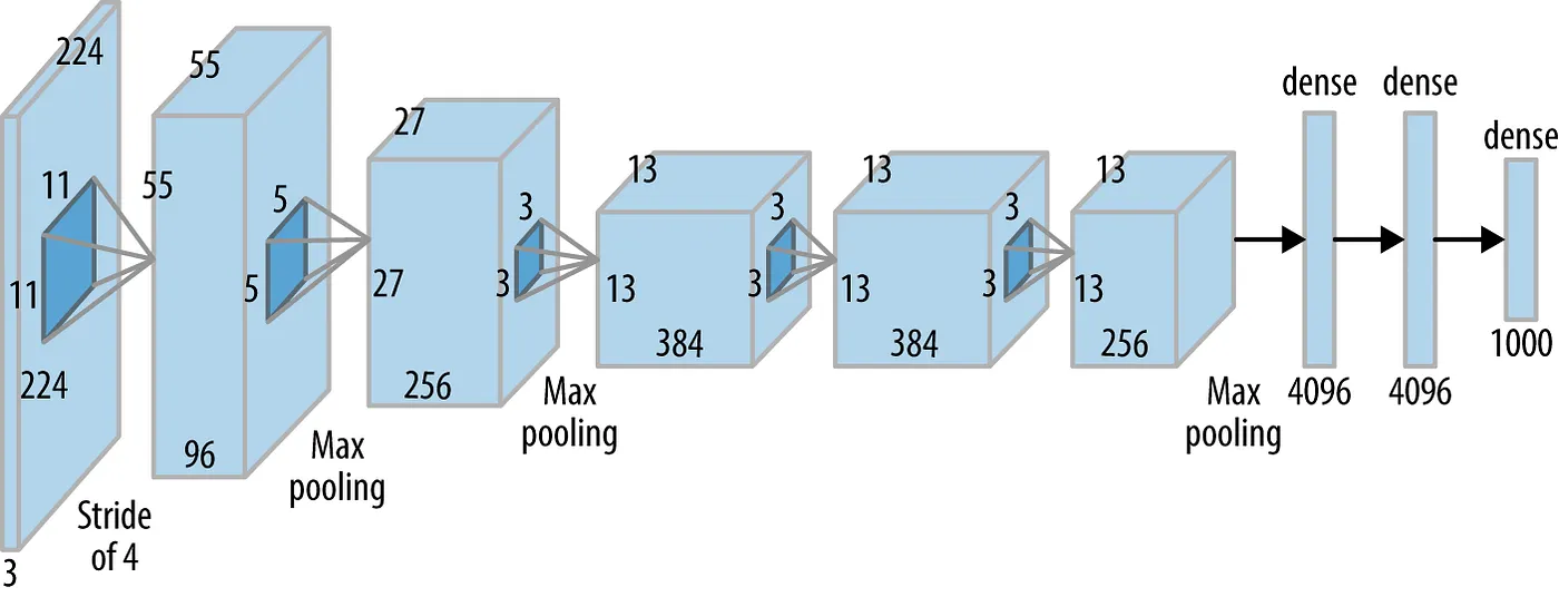
The network has a total of 62 million trainable variables

How? The input to the network is a batch of RGB images of size 227x227x3 and outputs a 1000x1 probability vector one corresponding to each class.

• Data augmentation is carried out to reduce over-fitting. This Data augmentation includes mirroring and cropping the images to increase the variation in the training data-set. The network uses an overlapped max-pooling layer after the first, second, and fifth CONV layers. Overlapped maxpool layers are simply maxpool layers with strides less than the window size. 3x3 maxpool layer is used with a stride of 2 hence creating overlapped receptive fields. This overlapping improved the top-1 and top-5 errors by 0.4% and 0.3%, respectively.
• Before AlexNet, the most commonly used activation functions were sigmoid and tanh. Due to the saturated nature of these functions, they suffer from the Vanishing Gradient (VG) problem and make it difficult for the network to train. AlexNet uses the ReLU activation function which doesn’t suffer from the VG problem. The original paper showed that the network with ReLU achieved a 25% error rate about 6 times faster than the same network with tanh non-linearity.
• Although ReLU helps with the vanishing gradient problem, due to its unbounded nature, the learned variables can become unnecessarily high. To prevent this, AlexNet introduced Local Response Normalization (LRN). The idea behind LRN is to carry out a normalization in a neighborhood of pixels amplifying the excited neuron while dampening the surrounding neurons at the same time.
• AlexNet also addresses the over-fitting problem by using drop-out layers where a connection is dropped during training with a probability of p=0.5. Although this avoids the network from over-fitting by helping it escape from bad local minima, the number of iterations required for convergence is doubled too.

VGGNet:

When?

• International Year of Family Farming and Crystallography
• First Robotic Landing on Comet
• Year of Robin Williams’ death

Why? VGGNet was born out of the need to reduce the # of parameters in the CONV layers and improve on training time.

What? There are multiple variants of VGGNet (VGG16, VGG19, etc.) which differ only in the total number of layers in the network. The structural details of a VGG16 network have been shown below.

VGG16 Block Diagram (source: neurohive.io)

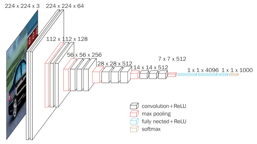
VGG16 has a total of 138 million parameters. The important point to note here is that all the conv kernels are of size 3x3 and maxpool kernels are of size 2x2 with a stride of two.

How? The idea behind having fixed size kernels is that all the variable size convolutional kernels used in Alexnet (11x11, 5x5, 3x3) can be replicated by making use of multiple 3x3 kernels as building blocks. The replication is in terms of the receptive field covered by the kernels.

Let’s consider the following example. Say we have an input layer of size 5x5x1. Implementing a conv layer with a kernel size of 5x5 and stride one will result in an output feature map of 1x1. The same output feature map can be obtained by implementing two 3x3 conv layers with a stride of 1 as shown below

Now let’s look at the number of variables needed to be trained. For a 5x5 conv layer filter, the number of variables is 25. On the other hand, two conv layers of kernel size 3x3 have a total of 3x3x2=18 variables (a reduction of 28%).

Similarly, the effect of one 7x7 (11x11) conv layer can be achieved by implementing three (five) 3x3 conv layers with a stride of one. This reduces the number of trainable variables by 44.9% (62.8%). A reduced number of trainable variables means faster learning and more robust to over-fitting.

ResNet

When?

• Discovery of Gravitational Waves
• International year of soil and light-based technologies
• The Martian movie

Why? Neural Networks are notorious for not being able to find a simpler mapping when it exists.

• For example, say we have a fully connected multi-layer perceptron network and we want to train it on a data-set where the input equals the output. The simplest solution to this problem is having all weights equaling one and all biases zeros for all the hidden layers. But when such a network is trained using back-propagation, a rather complex mapping is learned where the weights and biases have a wide range of values.
• Another example is adding more layers to an existing neural network. Say we have a network f(x) that has achieved an accuracy of n% on a data-set. Now adding more layers to this network g(f(x)) should have at least an accuracy of n% i.e. in the worst case g(.) should be an identical mapping yielding the same accuracy as that of f(x) if not more. But unfortunately, that is not the case. Experiments have shown that the accuracy decreases by adding more layers to the network.
• The issues mentioned above happens because of the vanishing gradient problem. As we make the CNN deeper, the derivative when back-propagating to the initial layers becomes almost insignificant in value.

ResNet addresses this network by introducing two types of ‘shortcut connections’: Identity shortcut and Projection shortcut.

What? There are multiple versions of ResNetXX architectures where ‘XX’ denotes the number of layers. The most commonly used ones are ResNet50 and ResNet101. Since the vanishing gradient problem was taken care of (more about it in the How part), CNN started to get deeper and deeper. Below we present the structural details of ResNet18

Resnet18 has around 11 million trainable parameters. It consists of CONV layers with filters of size 3x3 (just like VGGNet). Only two pooling layers are used throughout the network one at the beginning and the other at the end of the network. Identity connections are between every two CONV layers. The solid arrows show identity shortcuts where the dimension of the input and output is the same, while the dotted ones present the projection connections where the dimensions differ.

How? As mentioned earlier, ResNet architecture makes use of shortcut connections to solve the vanishing gradient problem. The basic building block of ResNet is a Residual block that is repeated throughout the network.

Residual Block — Image is taken from the original paper

Instead of learning the mapping from x →F(x), the network learns the mapping from x → F(x)+G(x). When the dimension of the input x and output F(x) is the same, the function G(x) = x is an identity function and the shortcut connection is called Identity connection. The identical mapping is learned by zeroing out the weights in the intermediate layer during training since it's easier to zero out the weights than push them to one.

For the case when the dimensions of F(x) differ from x (due to stride length>1 in the CONV layers in between), the Projection connection is implemented rather than the Identity connection. The function G(x) changes the dimensions of input x to that of output F(x). Two kinds of mapping were considered in the original paper.

• Non-trainable Mapping (Padding): The input x is simply padded with zeros to make the dimension match that of F(x)
• Trainable Mapping (Conv Layer): 1x1 Conv layer is used to map x to G(x). It can be seen from the table above that across the network the spatial dimensions are either kept the same or halved, and the depth is either kept the same or doubled and the product of Width and Depth after each conv layer remains the same i.e. 3584. 1x1 conv layers are used to half the spatial dimension and double the depth by using stride length of 2 and multiple of such filters respectively. The number of 1x1 conv layers is equal to the depth of F(x).

Inception:

When?

• International Year of Family Farming and Crystallography
• First Robotic Landing on Comet
• Year of Robin Williams’ death

Why? In an image classification task, the size of the salient feature can considerably vary within the image frame. Hence, deciding on a fixed kernel size is rather difficult. Lager kernels are preferred for more global features that are distributed over a large area of the image, on the other hand, smaller kernels provide good results in detecting area-specific features that are distributed across the image frame. For effective recognition of such a variable-sized feature, we need kernels of different sizes. That is what Inception does. Instead of simply going deeper in terms of the number of layers, it goes wider. Multiple kernels of different sizes are implemented within the same layer.

What? The Inception network architecture consists of several inception modules of the following structure

Inception Module (source: original paper)

Each inception module consists of four operations in parallel

• 1x1 conv layer
• 3x3 conv layer
• 5x5 conv layer
• max pooling

The 1x1 conv blocks shown in yellow are used for depth reduction. The results from the four parallel operations are then concatenated depth-wise to form the Filter Concatenation block (in green). There is multiple version of Inception, the simplest one being the GoogLeNet.

How? Inception increases the network space from which the best network is to be chosen via training. Each inception module can capture salient features at different levels. Global features are captured by the 5x5 conv layer, while the 3x3 conv layer is prone to capturing distributed features. The max-pooling operation is responsible for capturing low-level features that stand out in a neighborhood. At a given level, all of these features are extracted and concatenated before it is fed to the next layer. We leave for the network/training to decide what features hold the most values and weight accordingly. Say if the images in the data-set are rich in global features without too many low-level features, then the trained Inception network will have very small weights corresponding to the 3x3 conv kernel as compared to the 5x5 conv kernel.

Summary

In the table below these four CNNs are sorted w.r.t their top-5 accuracy on the Imagenet dataset. The number of trainable parameters and the Floating Point Operations (FLOP) required for a forward pass can also be seen.

Several comparisons can be drawn:

• AlexNet and ResNet-152, both have about 60M parameters but there is about a 10% difference in their top-5 accuracy. But training a ResNet-152 requires a lot of computations (about 10 times more than that of AlexNet) which means more training time and energy required.
• VGGNet not only has a higher number of parameters and FLOP as compared to ResNet-152 but also has a decreased accuracy. It takes more time to train a VGGNet with reduced accuracy.
• Training an AlexNet takes about the same time as training Inception. The memory requirements are 10 times less with improved accuracy (about 9%)

Bonus:

Compact cheat sheets for this topic and many other important topics in Machine Learning can be found in the link below

Cheat Sheets for Machine Learning Interview Topics

If this article was helpful to you, feel free to clap, share and respond to it. If want to learn more about Machine Learning and Data Science, follow me @Aqeel Anwar or connect with me on LinkedIn.